Fig. 1.
HRMAS spectra from normal mouse brain (C57/BL6) acquired at 37°C and 9.4 T (pulse-and-acquire sequence) with 6,000 Hz spinning rate, in 17 min. (a) Mouse euthanised with focused microwave (FMW) irradiation and (b) mouse euthanised with anaesthesia overdose. Note differences (arrows) in creatine (Cr, 3.93 ppm), phosphocreatine (PCr, 3.95 ppm) and lactate (Lac, 1.32 ppm) depending on the sacrifice method used. See Sect. 4.1 for further details.
In this respect, ample literature exists about using HRMAS as an ex vivo typing tool for human brain tumours (27–30), but much less for animal models of these brain tumours. For example, total spinning time has been shown to have non-negligible effects over the metabolome pattern (31) and even tissue architecture (32). Apart from this, varying tissue temperature produces mostly reversible pattern changes between 0 and 37°C, which do not seem to affect pattern recognition-based discrimination of major tumour types (33).
2 Technical Requirements for Successful MRSI and HRMAS Acquisition
The physiological and MRSI parameters herewith discussed will refer to studies carried out with mice, unless otherwise indicated.
2.1 Anaesthesia and Other Basic Monitoring Requirements for In Vivo MRSI
In order to obtain proper MRI/MRS/MRSI data, any movements during the MR exploration should be avoided. To achieve this, animals are usually explored under the effect of anaesthesia, which also reduces stress for the animal. General anaesthesia is a state of general depression of the CNS involving analgesia, suppression of reflex activity and relaxation of voluntary muscle. Convenient anaesthesia may be achieved both by means of inhalational and injectable agents. The main advantages of inhalational agents are that the depth of anaesthesia can be adjusted fast, animals recover from it quickly and agents used are either exhaled unchanged or metabolised only in relatively small proportions by the liver, therefore being less likely to interfere with experimental results (34). On the other hand, environmental pollution with inhalational anaesthetics must be considered a hazard to lab personnel and due precautions to avoid fully open administration methods should be considered. It is important to remark that both strain and genetic modifications in mice could cause variations in their susceptibility to anaesthesia-associated morbidity and mortality (35).
In our work, anaesthesia is always performed using isofluorane at 2.5–4.0% (induction in closed chamber) and 1–2.5% (maintenance with an open system) in O2 using an inhalational apparatus (Matrx VME2, Midkmark, Versailles, Ohio, USA). After induction, animals are moved to the Biospec 70/30 holder and MRI/ MRSI exploration is carried out as described in Sect. 3. During all experimental procedures, animals are always housed, handled and transported according to protocols previously approved by the institutional Ethics and Animal Welfare Committee and also according to regional and state legislation.
2.1.1 Monitoring Vital Signs
Minimal requirements for monitoring and physiologic support during anaesthesia depend on many factors including the health status of the animal, the anaesthetic employed and the objective of the imaging procedure. For example, more intensive monitoring and support would be indicated for an animal weakened by prior experimental manipulations, especially when undergoing lengthy functional imaging procedures (36).
Temperature Control
Differences between ambient and body temperature must be minimised, since the hypothalamic heat-regulating mechanism is depressed during anaesthesia and the animal is no longer able to shiver. As rodents have large surface area to body mass ratio, heat losses will be correspondingly greater than in bigger animals (34). Low body temperature has profound effects in modifying drug activity, although in some cases it might exert a protective effect, particularly in the CNS, that may be wise to consider (21, 34). This fact has been put to effective use in protecting organs whilst the blood supply is temporarily suspended. Body temperature can be monitored with rigid or flexible probes, which are available in multiple sizes allowing their use with small rodents including mice. Temperature probes most frequently are placed in the rectum. The usual rectal temperature in mice is 37.5°C (35.5–39°C) (34).
A self-regulating heating device generally consists of three units: a probe, a temperature controller and a warming source (such as a warm water recirculating blanket). Changes in the body temperature are then automatically adjusted for by altering the temperature of the warming source, thereby maintaining the animal within a very narrow temperature range (36). In our case, a heated water blanket incorporated into the MR system is used to avoid hypothermia and/or control the desired temperature, in case that a moderate hypothermia is desired. In studies carried out at normothermia, temperature is maintained between 36.5 and 37.5°C. On the other hand, in studies carried out with moderate hypothermia, the body temperature is adjusted to 28.5–29.5°C. In case finer local temperature monitoring for brain is required, this may be achieved by MRSI as described in Sect. 3.6.
Breathing Rhythm Control
Most agents which depress CNS activity are also respiratory depressants (36, 37). Essential organs, particularly the CNS and liver, may be severely damaged by relatively brief periods of O2 deprivation and the respiratory depression during spontaneous breathing usually becomes irreversible when it falls to about one-third of the normal rate (34). The respiratory frequency is usually evaluated by counting breaths per minute. The physiological breath rhythm expected for an awake mouse is 160–180 breaths/min (range 80–100 to 230–250) (34, 37). Changes in breathing and, consequently, in oxygenation can affect results, especially during functional imaging, by altering drug metabolism or cerebral blood flow. Respiratory rate can be approximated through chest movement detected by a small compressible pillow integrated with a pressure transducer. The animal’s respiratory movement compresses the pillow and affects the pressure transducer that is linked to a computer that provides a graphical display of movement and the calculated respiratory rate. The respiratory rhythm in our experiments with anesthesized mice is maintained at 60–80 breaths/min.
Both temperature and breathing rhythm are monitored by a control/gating module from SA Instruments Inc. (Stone Brook, NY, USA). Data gathered by the module are transferred to a personal PC (Dell Inspiron 510m) and monitored with the PC-SAM 32 software (version 6.26, Small Animal Instruments, Incorporated).
2.1.2 Post-anaesthetic Management
Too often, there is a swift decrease in the attention devoted to the animal as soon as the experimental procedure is completed, when there is still considerable risk of animal death. Careful attention must be paid until the animal is fully conscious. A warm recovery environment is essential and should be prepared before the animal is anaesthetised. This assumes that body temperature is normal at the time of anaesthetic procedures. If the animal is allowed to become hypothermic, the metabolic rate will be correspondingly depressed and recovery may be delayed by slow detoxification of the anaesthetic agent (34). Also, we should pay attention because in our case, preclinical models of brain tumours, the animals are not in their optimum health state. Biological systems which are already subject to pathological changes may be particularly affected by anaesthesia, and this is more pronounced during long anaesthesia periods as usually needed for combined MRI/MRSI experiments. In our experiments, animals are maintained in a warm environment and monitored until total recovery (usually between 5 and 7 min), and after that period they are returned to their cage.
3 Recording Strategies for MRSI Experiments
In Sects. 3.1 through 3.4, specific details are provided on how to acquire highly resolved 1H-MRSI data from preclinical mouse models of human brain tumours, while Sect. 3.5 considers post-processing requirements. In Sect. 3.6, hyperpolarised 13C-MRSI is briefly considered, dynamic versus basal MRSI discussed and MRSI thermometry described.
3.1 1H-MRSI: Shimming Quality, Water Suppression, Volume of Interest Selection, k-Space Sampling and Echo Time
The principles of 1H-MRSI are very similar to those of MRI as far as phase encoding and basic pulse sequences. The main difference is an additional frequency axis—the chemical shift dispersion (Figs. 2 and 3). Hence MRSI is often called chemical shift imaging or CSI. In vivo 1H-MRSI of the brain is challenging for four main reasons: large signals, like extracranial lipids, can overwhelm small metabolite signals; the water resonance is several orders of magnitude larger than signals produced by the low concentration of metabolites (often more than 10,000 times); its low sensitivity makes the detection of low concentration metabolites a compromise between time resolution and signal-to-noise ratio (SNR) and there is a large overlap between different metabolite resonances. To overcome the first two problems, at least partially, efficient spatial localisation and water suppression methods are required, respectively.
Fig. 2.
Single voxel (SV) 1H-MRS (on the left, red contour line) and 1H-MRSI (on the right, blue contour line) obtained from a normal C57BL/6 mouse brain in vivo, with PRESS localisation, at 7.0 T. The upper panel shows (small centre inset) a reference T2-W image of the brain and the PRESS voxel positions, in the centre of the FOV: 1H-MRS, 27 μL voxel volume; 1H-MRSI, 4.8 μL nominal voxel size, Fourier interpolated to 0.3 μL as displayed. Data were acquired with TR/TE = 2,500/12 ms, VAPOR water suppression and outer volume suppression. Details about resonance assignment can mostly be obtained from (103). Ala alanine, Cho choline, Cr creatine, GABA γ-aminobutyric acid, Gln glutamine, Glu glutamate, Ino myo-inositol, Lac lactate, MM macromolecules, NAA N-acetyl aspartate, NAAG N-acetylaspartyl glutamate, PCr phosphocreatine, Tau taurine.
Fig. 3.
1H-MRS and 1H-MRSI obtained in vivo at 7.0 T from two C57BL/6 brain tumour-afflicted mice: (a) spontaneous grade 2 oligodendroglioma detected in a genetically engineered mouse model: s100ß-v-erbB;Ink4a/Arf(+/−) (22); (b) high grade IV astrocytoma detected in an allograft model, intracranial stereotactic injection of GL261 cells. For (a) and (b), SV 1H-MRS at different TEs (12–136 ms) with T2-W reference image on upper-left showing the SV MRS voxel position (red square). 1H-MRSI, at 12 ms TE, with 10 × 10 voxels within the VOI region is also highlighted on the T2-W reference image (blue square); spectra highlighted with red squares over the enlarged MRSI matrix, bottom-left in (a) and (b), are also enlarged on the right-side and correspond to normal/peritumoural brain and tumour (1 and 2, respectively). SV voxel in (a) and (b) have square and rectangular shapes, respectively.
Restricting signal detection to a defined region of interest, usually named volume of interest (VOI) for 1H-MRSI (voxel for 1H-MRS), has several advantages. Not only it removes unwanted signals from the outside and minimises partial-volume effects (contamination of signal from one compartment by signal from another compartment) but also reduces B 0 and B 1 field variations within the region of interest, allowing better resolved spectra to be obtained. The standard technique for in vivo 1H-MRSI localisation in preclinical and clinical settings is PRESS (point resolved spectroscopy) (38), although STEAM (39) is also used to acquire 1H-MRS(I) data (6, 21). Other methods have also been described to achieve MRSI voxel localisation, taking advantage of adiabatic RF pulses (40–43) and used for mouse brain MRSI (7).
To improve SV localisation, it is sometimes important to remove unwanted magnetisation outside the field of view (FOV), i.e. to perturb this magnetisation while leaving the magnetisation in the VOI unperturbed during the localisation procedure. This is normally named outer volume suppression (OVS), and it is used in the MRSI studies described in this chapter. Since water is the most abundant compound in mammalian tissue, it is no surprise that its two protons dominate the individual 1H-MRSI patterns in the region where they resonate (ca. 4.75 ppm). This also leads to baseline distortions and artefacts, i.e. water sidebands due to vibration-induced signal modulation, which compromise the detection of certain metabolite resonances. Therefore, it is necessary to remove or suppress the water resonance in order to obtain reliable metabolite spectra. Although there are different techniques available to achieve this, two of the most commonly described in the literature are CHESS (chemical shift selective “water suppression” (44, 45)) and, more recently, VAPOR (variable pulse powers and optimised relaxation delays (46)). VAPOR essentially combines T1-based water suppression, i.e. uses T1 relaxation to discriminate between water and other resonances, and optimised frequency-selective perturbations, to provide excellent water suppression with a large insensitivity towards T1 and B 1 inhomogeneity.
As far as acquisition, two basic parameters are important in any MR spectroscopy technique: the number of scans, i.e. number of times that the sample is excited and the signal is recorded (free induction decay or FID); and the repetition time (TR), i.e. the interval between consecutive scans during the experiment, when the nuclear spins generate the MR signal (FID), and are allowed to relax, which defines the total duration of each experiment. In the specific case of in vivo localised MR spectroscopy, the transversal relaxation of the nuclei due to intrinsic sample and instrumental causes is too fast to allow recording a usable FID, and another parameter comes into play—the echo time (TE). This is the same as in standard spin-echo MRI sequences, such as RARE, and basically refers to the time elapsed between excitation of the nuclei and their refocusing for recovering most of the initially lost signal. By choosing specific values for this parameter, one can select the brain molecules seen on the spectral profiles according to their intrinsic T2 values and possible J-couplings, e.g. filtering out most MR-visible lipids (frequently abundant in tumours) or allowing to observe the characteristic inversion of Lactate at 1.32 ppm due to J-coupling-induced modulation at long echo times of 135–144 ms.
All of the above applies both to MRSI and to conventional MRS. MRSI is, however, much more technically demanding than MRS, essentially due to: significant magnetic field inhomogeneities across the entire sample, particularly in the mouse brain as compared, e.g. to the rat brain; spectral degradation due to intervoxel contamination (“voxel bleeding”); long data acquisition times and processing of large, multidimensional datasets (2D, 3D or even 4D). Concerning magnetic field homogeneity adjustments (shimming, a process that consists in adjusting the current at a series of small coils placed around the sample area), fully automated procedures based on B 0 mapping have been described (47, 48) which considerably reduce the time and effort during this procedure while producing excellent results. With respect to intervoxel contamination, this is a typical problem in Fourier imaging modalities and results from the Cartesian sampling of k-space. This contamination in MRSI spectra from adjacent voxels is explained by the shape of the spatial response function (SRF, displays the spatial origin of the signal of a pixel) which is not square but, instead, a sinc-like function (49). It has been described, however, that acquisition-weighted CSI, a non-Cartesian method of sampling k-space, consisting in applying a k-space filter, e.g. Hanning window, which gives more weight to the phase-encode steps at the centre of k-space than to those in the outer regions, reduces this contamination substantially with no penalty in sensitivity or spatial resolution (2, 50).
The next sections describe how to acquire highly resolved PRESS 1H-MRSI data from the mouse brain, or mouse brain tumours, using acquisition-weighted sampling of k-space. An outcome example is provided in Fig. 3.
3.2 1H-MRSI, Hardware
The following hardware and software configuration is advised in order to acquire routinely good quality 1H-MRSI data from rodent brains, in particular, from the mouse brain and mouse brain tumours:
1.
A high-field magnet, at least 7 T, preferably horizontal.
2.
Robust gradient and shim systems, with at least 300 mT/m and nine channels, respectively, capable of handling high duty cycles (strong shim currents).
3.
A proton mouse head RF coil with good SNR, e.g. receiving quadrature surface coil decoupled from a transmitting resonator.
4.
An anaesthesia induction chamber, with anaesthetic gas circulation (e.g. isoflurane) and proper exhaustion system.
5.
A robust animal holder, allowing efficient head restraining (stereotactic type, with fixation points at both ear cavities and a biting tooth bar), optimal circulation of anaesthetic gas (e.g. isofluorane) and body temperature control (e.g. recirculating heated water system).
6.
Medical tape, eye lubricant and vaseline.
7.
Real-time monitoring of basic physiologic parameters of the animal, specifically the respiratory rate with, e.g. chest/abdominal sensor, and the body temperature with, e.g. rectal probe; see Sect. 3.4. for additional comments.
8.
Automated protocol(s) for localised adjustment of first- and second-order shims.
9.
The MRSI protocol, including,
Spin-echo acquisition mode.
Hanning filter for phase encoding steps.
PRESS localisation.
VAPOR water suppression.
Protocols for standard anatomical MRI sequences are also required but normally available in any commercial MR spectrometer.
3.3 1H-MRSI, Protocol
The following protocol describes all the steps required to generate highly resolved 1H-MRSI data from the mouse brain and mouse brain tumours, as reported (21), i.e. using a Bruker 70/30 BioSpec magnet running with Paravision 4.0 software.
1.
The animal is moved from its cage to the anaesthesia induction chamber, where isoflurane gas mixture (4% in O2, 1 L/min, for about 1 min) is used to put it to sleep.
2.
The animal is transferred, while asleep, to the MR holder (should be performed fast), where isoflurane is already circulating at 1.5–2% and 0.8 L/min, and water, heated at about 50°C (depends on the specific configuration used and should be adjusted to keep the body temperature at 37°C unless otherwise indicated), is also circulating.
3.
The animal is placed in the MR holder, as detailed in Fig. 4 and Sect. 3.4, and pushed inside the magnet in a way that the brain (tumour lesion) rests in the iso-centre.
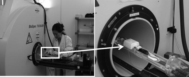
Fig. 4.
(Left) Overview of the animal holder used for preclinical studies (mice) in the Biospec 70/30 scanner. (Right) Detail of the animal holder with the surface coil positioned.
4.
The PRESS 1H-MRSI protocol is loaded after syntonising the probe and acquiring standard multislice and multidirection localisation MRI scans.
5.
The acquisition-weighted mode is selected (Hanning window) and the acquisition and reconstructed MRSI matrix sizes are defined (e.g. 8 × 8 and 32 × 32, respectively).
6.
Select VOI visualisation mode and position the VOI box in transversal plane (e.g. 5.5 × 5.5 mm in-plane and 10 mm thickness) in the brain region of interest, using the localisation MRI scans.
7.
Change to FOV mode and position the FOV window (e.g. 1.76 × 1.76 cm in transversal plane and 1 cm slice thickness) in a way that it covers most of the animal head and includes the VOI inside the brain region of interest and without reaching the skull.
8.
Load a RARE T2-w sequence, use the same FOV geometry and position as in the MRSI experiment, and acquire it—this will be the MRSI reference image.
9.
Go back to the MRSI experiment and select six OVS slices, two for each plane with 10 mm thickness each (sech-shaped pulses: 1.0 ms/ 20,250.0 Hz), and position them all around the VOI (Fig. 5).
Fig. 5.
The six OVS slices (two for each plane, transversal, sagital and coronal) overlaid on a scout MR image.
10.
Load a FASTMAP experiment, position its voxel (e.g. 5.8 × 5.8 × 5.8 cm for mice) inside the brain in a way that includes the VOI and carry out the automatic linear and second-order shim adjustments.
11.
Load a PRESS-MRS experiment, with the same geometry and position as the MRSI VOI, run an additional adjustment of first-order shims (this time specifically inside the VOI region), optimise PRESS pulse powers (hermite-shaped pulses: excitation, 0.6 ms/ 9,000 Hz; refocusing, 0.6 ms/ 5,700 Hz) previously used for MRSI, and acquire a single scan of non-suppressed water signal using the TR, TE, spectral width and number of points in the time domain chosen for MRSI (e.g. 2.5 s, 12 ms, 4,006.41 Hz (13.34 ppm) and 2 k, respectively)—expected waterline widths at half height should be as low as possible, and normally around 15–22 Hz (if higher try to reposition the VOI and re-shim).
12.
Go back to the MRSI experiment, turn on water suppression and adjust VAPOR pulses (hermite-shaped pulses: excitation, 18.0 ms/300 Hz; 11.4 ms, 300 Hz)—see Sect. 3.3.
13.
Define number of scans (e.g. 512) and dummy scans (e.g. 4), and acquire.
14.
The reconstruction pipeline (see also Sect. 3.5) should automatically Fourier interpolate the FID signal acquired to the reconstructed matrix size, defined in step 5.
This protocol, and orientative values provided thus far, will generate 1H-MRSI data with nominal spatial resolution of 2.2 mm, i.e. 4.84 μL voxel volume, and, after post-acquisition automated Fourier interpolation, digital in-plane voxel sizes of 0.55 mm, i.e. 0.30 μL—see Sect. 3.3. In case artefacts are detected in the individual spectral patterns, these may be due to the spoiler gradients, which crush the residual magnetisation at the end of each scan. If so, they should be adjusted (intensity and/or duration) to minimise those artefacts.
3.4 1H-MRSI, Useful Considerations
Other parameters, such as heart rate (with, e.g. finger paws) or expired gases (e.g. CO2), may also be of interest to monitor, depending on the experimental procedure being carried out.
The mouse head is fixed without forcing any of the bars; a lubricant jelly is applied directly into the eyes to prevent them from drying throughout the experiment; a rectal probe is lubricated (Vaseline) and inserted into the anus for body temperature monitoring; the animal can be covered with standard laboratory bench paper to help prevent heat losses, along with the heating water system.
VAPOR pulses (gains) should be adjusted until achieving maximum suppression of the water peak; however, for post-processing generation of certain maps, e.g. temperature (detailed in Sect. 3.6), spectra should only be partially water-suppressed, so that the residual water signal is clearly visible throughout the VOI region.
Due to the non-Cartesian sampling of k-space (acquisition-weighting), the original MRSI signal is acquired beyond the FOV limits, from a grid determined by the Hanning window (13 × 13 in the case described in this protocol: 12 accumulations in the centre of k-space; total of 113 phase encoding steps). Hence, at least one interpolation step (Markus von Kienlin, personal communication) is required to properly visualise the data acquired inside the FOV.
3.5 Post-processing for MRSI
3.5.1 Producing MRSI Maps: Options Available
After successful application of the acquisition protocols described in Sect. 3.3 to living mice, similar MRSI grids to those shown in Figs. 3 and 6 can be obtained.
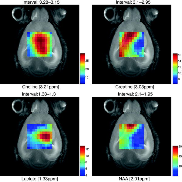
Fig. 6.
Metabolite maps superimposed over a T2 reference image in a C57 mouse (code number, C69) bearing a GL261 tumour, from MRSI acquired at long TE (136 ms) obtained using the SC3.0 software and the other modules available from http://gabrmn.uab.es/ (see text). The colour scale to the right of each plot shows the relative intensity, in absolute value, of each peak height analysed from unit length normalised spectra (UL2, (74, 105)) (choline, creatine, lactate and NAA; the interval above individual figures indicates the ppm range where the absolute peak maxima were located by the software, see Sect. 3.5.1). It can be seen that different metabolites have a distinct distribution in the grid, hence in the tumoural (high choline, high lactate), peritumoural or non-affected areas (high NAA, high creatine).
The interpretation of one of these grids (about 100 spectra) superimposed to a brain image is however, not straightforward, let alone the assignment of metabolites to peaks and their quantification. Therefore, performing this step by visual inspection alone on a regular basis is not feasible. It is strongly recommended that each MRSI grid is visually inspected by the operator just after having performed the experiment, in order to identify whether there is any evident artefact and to decide whether the acquisition should be repeated or not. A good guide to MRS artefacts can be found in (51). In general, the aim is to obtain an MRSI grid in which all spectra are well resolved (good shimming), have good SNR (enough number of accumulations), water suppression is well achieved (pulses well calibrated) and no outer volume contaminations are detected in the individual MRS patterns. The latter are frequently found in PRESS-MRSI of the brain, such as “ghost” artefacts and lipid contamination from the skull (51), and can be compensated by adjusting the crusher gradients and OVS pulses, as well as by keeping the VOI away from the skull.
Once the experimenter has ensured that the MRSI is of sufficient quality, interpretation should follow. To do that, the most common methods consist in obtaining metabolite or metabolite ratio maps. Metabolite maps are images in which colour intensities encode either the spatial distribution of a certain metabolite peak (2, 3, 5) or alternatively, intra-voxel ratios of selected peak intensities. The latter option may be used within the same MRSI grid, to compare different metabolites, e.g. choline/creatine or NAA/choline (21, 52–54), or to monitor time-course changes of a specific metabolite (55).
Alternatively, maps of normalised intensities can also be generated to have a quick overview of the metabolite distributions over the MRSI grid (Fig. 6). Whatever method is chosen, the best way to interpret a metabolic map is to overlay it on a reference MR anatomical image, with the same geometry and position as the MRSI scan. Some examples are shown in Fig. 6 for brain tumour-bearing mice.
When there is an underlying pathological state, it is expected that the spatial distribution of the different metabolites will not be homogeneous (7, 56–58) and the metabolite map of specific metabolites will have different intensities. These intensities will colocalise with certain areas, such as diseased or injured ones (1, 3, 59) (Fig. 6).
Maps of dynamic metabolite changes (21) can provide additional information about the tumour progression stage (type and grade) and its heterogeneity.
As it can be seen in Fig. 6, depending on the metabolite map represented, the image changes and it is self-evident for an experienced biochemist that all these maps give complementary information to delimitate the tumoural or the unaffected brain tissue. But none of those in fact, unequivocally segment the abnormal area. Why then not try using the information provided not by one metabolite but the entire spectral pattern at the same time, in all voxels, to make a map? To meet this end, MRSI data analysis may also be performed by pattern recognition (60, 61). Pattern recognition is a statistical technique for multivariate analysis which allows analysing several peak areas or heights at the same time (i.e. several variables) and weighs them according to a statistical formula. Pattern recognition, therefore, aims to assign, in an objective way, output values (i.e. tissue type, pathologic state) to certain input features, e.g. the peaks in a 10 × 10 MRSI grid. Generally speaking, pattern recognition methods can be divided into supervised and unsupervised. Unsupervised methods, such as principal component analysis (PCA) have been, and still are widely used, but we prefer supervised approaches, such as linear discriminant analysis (LDA). Unsupervised methods are a good choice for performing an initial analysis of the data, but are not well suited for predicting these output values on a new dataset (test set) on the basis of a previous set of data of known class (training set).
Therefore, imaging tumours based on objective classification of MRSI data brings us closer to the long-pursued concept of nosologic imaging (62). A nosologic image is one in which the presence of different tissues and lesions is summarised in a single, colour-coded image, where each pixel or voxel is coded according to its histopathological class (the output value) (63). This methodology is well reported for human tumour MRSI data (64, 65) and has been shown to be feasible in animal models (12, 13, 66). In this way, a classification image would be a general term with which we simply designate the image produced after classification, i.e. two-colour images of “normal brain vs. abnormal brain,” or “brain vs. ventricles,” whereas a nosologic image would be more appropriate when talking about tumours, in which the pathological diversity of the tissue is taken into account, i.e. a three-class classification image for “necrosis vs. high-grade glioma vs. low-grade glioma.”
But generating the MRSI maps described in Sect. 3.5.1 requires access to advanced processing and post-processing software tools. Several options are available, either from manufacturer providers, e.g. ParaVision (Bruker), or released by specific research groups. Some examples of advanced multipurpose NMR processing software include: LC Model (67), jMRUI(68), CSIAPO (63), 3DiCSI (http://mrs.cpmc.columbia.edu/3dicsi.html) that allow reading data from different manufactures, and allow overlying MRSI data, either 2D or 3D, on MRI reference scans. jMRUI (AMARES and QUEST) and LC Model are two of the most popular tools for quantification of MRS data (68). These software tools are based on time- and frequency-domain analysis of the data, respectively, allowing line-fitting and deconvolution of the spectral peaks detected. Another option for carrying out individual line-fitting integration of MRSI data is XSOS (69). Other post-processing tools, such as dynamic MRSI processing module (DMPM) (http://gabrmn.uab.es/dmpm) for alignment, normalisation and map generation, and SpectraClassifier (70) (http://gabrmn.uab.es/sc) for performing pattern recognition analysis were developed by our research group and are free. Pattern recognition can also be performed with standard programs such as R (http://www.r-project.org/) or Matlab (http://www.mathworks.com/products/matlab/) and its toolboxes, but using these requires of a previous learning curve of a set of basic commands and is not suitable for those not familiar with these types of interfaces or with scarce time. The SpectraClassifier interface was designed to meet the needs of a typical biochemist with no special expertise in these programs.
3.5.2 MRSI Post-processing Protocol
The steps we follow for producing maps like those shown in Fig. 6 are detailed below.
Get Clinical Tree app for offline access
1.
Fourier interpolate the original MRSI matrix to 32 × 32 voxels with ParaVision 4.0 or 5.0 (see Fig. 7) or directly with CSIAPO by voxel shifting, both enabling line broadening adjustments, with a 4 Hz Lorentzian filter, and zero-order phase correction. The result will be an ASCII file containing the processed MRSI.
Fig. 7.
Diagram of the post-processing strategy used to generate colour-coded maps from MRSI scans.
2.
Feed the ASCII file into an additional post-processing module, DMPM (http://gabrmn.uab.es/dmpm), to ensure proper alignment and to produce metabolite and metabolite ratio maps.
3.
It is very important to normalise the spectra prior to classification. We take the 4.5–0 ppm region of each spectrum and normalise it individually to unit length (UL2), as previously described (55), with DMPM, prior to exporting for classification.
4.
Load the aligned, normalised spectra into the SpectraClassifier software, to classify the individual voxels in one or several MRSI grids.


(a)
Build the training set, i.e. the dataset that will be used to train the classifier. For this, it is necessary to tag each spectrum in each MRSI grid that is to be loaded (Fig. 8).
Fig. 8.
An easy example in which classification between normal brain tissue and tumour is performed. The training set is composed of four mice (C209, C234, C241 and C245), injected with GL261 glioblastoma cells, and the test set of two additional mice (C290 and C292). The four MRSI grids are tagged according to the reference MRI: blue, normal/peritumoural brain parenchyma; red, tumour. A classifier is obtained based on these data and then tested with the two additional mice: light blue, normal/peritumoural brain; yellow, tumour.
(b)
Build the test set, i.e. the dataset that the user wants to predict, e.g. the MRSI of one or more different new mice. It is very important that both training and test sets have been obtained under the same experimental conditions and that post-processing has been done in exactly the same way. Otherwise, different number of points or different point/ppm ratios, or different normalisations may produce unreliable results.
(c)
Perform feature selection. Do not overtrain the classifier. Overtraining is easily recognised when a near-perfect classification performance in the training set drops to less than chance in the test set. This is normally caused by using too many features for a small sample, which is called “the curse of dimensionality” (71). A rule of thumb for an ideal feature number is to use no more than one-third of the number of cases available for training (72).
•Perform classification. Evaluate results both in the training and in the test set. Receiver-operating curves (ROC)(73) and bootstrapping, as well as confusion matrices, are good tools for this. Repeat the process as many times as needed, changing the number of features in order to obtain the best classification results both in the training and in the test, with the minimum number of features. If the aim is to obtain the best classifier and the test results are not needed for any immediate reason, the following trick can be used (74): Divide all MRSI in two sets of approximately equal size.
•Use set 1 for training and set 2 for testing. Evaluate results.
•Use set 2 for training and set 1 for testing. Evaluate results.
(d)
If results are comparable, both with respect to the classification performance and the features chosen, the classifier is representative of the whole population.
Stay updated, free articles. Join our Telegram channel
Full access? Get Clinical Tree
