, Christopher R. Pryce2 and Erich Seifritz3
(1)
Wellcome Trust Centre for Neuroimaging, University College London, 12 Queen Square, London, WC1N 3BG, UK
(2)
Preclinical Laboratory for Translational Research into Affective Disorders, Clinic for Affective Disorders and General Psychiatry, Psychiatric University Hospital Zurich, Zurich, Switzerland
(3)
Clinic for Affective Disorders and General Psychiatry, Psychiatric University Hospital Zurich, Zurich, Switzerland
Abstract
Uncertainty is an important concept in neuroscience: due to its relevance in everyday life, because of theoretical significance for neurocomputational models, and clinical implications. A body of empirical research has tackled fundamental questions about how uncertainty is represented in the brain and what impact it has on behaviour. In this chapter, we review how uncertainty on different variables can be studied in isolation and how it can be quantified. Building on theoretical and empirical work that has been carried out so far, we propose rigorous experimental designs that should help in testing and understanding uncertainty and its translational relevance to adaptive behaviour and affective disorders.
Key words:
Uncertaintyentropyvarianceprobabilistichierarchicalcognitive neurosciencefunctional neuroimagingfMRIMEGpsychiatry1 Introduction
Research about uncertainty has received increasing interest over the last decades. Indeed, uncertainty is one of the main constants in life. For any organism, nothing is ever certain. Any perception, any representation of external states, or any computation bears imprecision. Humans often have a conscious notion of this uncertainty, humans and animals behave as if they know about it, and behaviour has been shown to be more optimal when uncertainty is taken into account. This has raised the question of whether there is a specific representation of uncertainty in the brain and how and where this is organised. Such research questions embrace a clinical perspective which posits that, for example, disorders in the schizophrenic spectrum are characterised by a fundamental misrepresentation of uncertainty, arising through increased stochastic noise in neural circuits (see, e.g. 1), and on a higher cognitive level, maladaptive styles of coping with uncertainty could be crucial, for example, in generalised anxiety disorder (see, e.g. 2).
The bulk of uncertainty literature, starting in the 1950s and 1960s, takes the form of research into the effects of a situation where, e.g. aversive events are uncertain, or unpredictable, as opposed to another situation where they are certain, or predictable. This view posits discrete psychological states associated with the presence, or absence, of uncertainty and has advanced our understanding of clinical conditions such as depression and anxiety. It does, however, not address the fact that uncertainty is ubiquitous and its fundamental role in guiding (and possibly misguiding) behaviour.
This role is acknowledged by more recent research topics which evolved from areas as diverse as behavioural economics, theoretical neuroscience and machine learning. They try to pin down how uncertainty on many different quantities is detected, represented in the brain and used to guide optimal behaviour. These approaches require a finer understanding, and more careful experimental manipulation, of uncertainty, where the fundamental issue is its definition and quantification.
An exhaustive theoretical treatment of uncertainty is beyond the scope of this chapter. Here, we seek to summarise existing approaches, and make them available to interested researchers, by giving a brief introduction into fundamental concepts of uncertainty from probability theory, reinforcement learning, perceptual decision-making and economics. Some of the distinctions and definitions we make may be perceived as subtle, but they pertain to very fundamental issues of brain function and can be exciting to study.
Several computational theories of brain function are based on probabilistic concepts and thus naturally account for uncertainty on many levels at the same time. They are based, for example, on the framework of predictive coding or on empirical Bayes methods (see sensorimotor control theory (e.g. 3), models of visual cognition (e.g. 4), the free energy principle (5), and others). Drawing on such theories, one can freely vary sensory inputs and estimate uncertainty on different quantities. Such estimates can then be related to measured brain functions or behaviour. However, this strategy rests on the assumption that the model one is using accurately describes brain function, which is necessarily speculative. This motivates the need for the isolated investigation of different forms of uncertainty. In this approach, one seeks to vary uncertainty on one quantity and carefully keep it constant on other quantities. This is the approach that we propose here. It revolves around two central premises:
(1)
There is no unitary account of uncertainty – uncertainty is always about something, and it can be about different things. What we are uncertain about is important because it shapes the way behaviour is organised. For example, the occurrence of electric shocks with uncertain onset might make it optimal to move as little as possible in order to save energy (i.e. freezing in context conditioning) (6). On the other hand, the presence of a shadow at night with uncertain significance might require approaching it and having a closer look (i.e. risk assessment behaviour) (7). On a neuronal level, it has been proposed that uncertainty is coded in a common way for different variables we are uncertain about: population coding (i.e. uncertainty is represented in the pattern of a neural population) (8), fixed-form coding (i.e. uncertainty is directly represented as a discrete quantity) or implicit coding (i.e. uncertainty is calculated from the mean of some quantity) (5). However, if such a common principle exists, it will probably be implemented in different brain areas and neurotransmitter systems, and bear different behavioural consequences, depending on what we are uncertain about.
(2)
Uncertainty can be quantitatively measured – therefore experiments on uncertainty can and should continuously manipulate uncertainty along a continuum from low to high, instead of contrasting it with certainty. Although the latter approach has many merits and forms the bulk of literature in many areas, uncertainty often is a psychologically salient feature such that a direct contrast of uncertainty and certainty encompasses processes that are theoretically unrelated to uncertainty. As an example, we have recently shown that brain responses that appeared to be caused by uncertainty about outcome contingencies (9) were not strongest when uncertainty was highest. Instead, they only occurred when it was made clear to subjects that the (uncertain) outcome rule was pre-determined and hidden, such that it was known with certainty to the experimenter, perhaps implying that it was thus potentially knowable for the subject as well. This points to social factors and qualitative behavioural strategies as key sources for this brain activation and demonstrates that the direct contrast of uncertainty with certainty can be difficult to interpret (10, see for a discussion (11)). Recent attempts have been made to disambiguate a categorical manipulation of uncertainty from confounding variables (12), however, it seems more promising to investigate uncertainty by experimentally varying it continuously. Not only does this provide a dose–response relationship; but it also forces the researcher to conceptualise why uncertainty should be represented in the brain and by which statistical rule. This provides for a deeper understanding of the underlying processes than a merely phenomenological approach.
2 Uncertainty in a Hierarchical Model of Action
For every quantity represented anywhere in the brain, we can define and investigate its uncertainty. In order to make this chapter tractable, we group related uncertainty manipulations into four levels of a decision-making process; the idea is to give a heuristic framework while acknowledging that these groups do not form exclusive or coherent processing levels.
If we imagine an action episode, uncertainty can arise at various stages. In the first place, perceptual information needs to be processed to provide relevant information. At night, we might be uncertain about what we see. Such perceptual uncertainty thus arises, for example, from incomplete sensory information or lack of attention. Next, perceptual information is used to infer facts about the situation we are in. Are we on a busy road in London, or in New York or at a friend’s party? Uncertainty about the state (or context) can put us into uncomfortable situations, as the context often prescribes certain rules according to which we behave. But are we certain about these rules? This might be the first party we attend in a town we recently moved to, and even though we know where we are, that does not imply that we know precisely how to behave. Uncertainty about rules is a typical initial condition in reinforcement learning. But then, at the end of learning, we might still not precisely know what is going to happen when action outcomes are probabilistic. Even if we know that a coin flip will result in tails half of the time, we do not know what the result of the next coin flip will be. Such outcome uncertainty is commonplace in everyday life.
Thus, a real-life stream of actions can often be broken up into small episodes to which the hierarchical model presented here can be applied. The central idea is that uncertainty on different levels of the hierarchy might be implemented by different neural mechanisms, such as different brain areas, networks or transmitter systems; but that related quantities might be represented in a similar manner. Therefore, it seems plausible to group similar forms of uncertainty and present them together: (1) perceptual uncertainty, i.e. uncertainty in the sensory information or its interpretation; (2) state uncertainty, i.e. uncertainty about which of several sets of (known) rules apply in a given moment, including uncertainty about the context and about state transitions; (3) rule uncertainty, i.e. uncertainty about stimulus–outcome or stimulus–action–outcome rules as such; (4) uncertainty about probabilistic outcomes, where outcome is defined as a motivationally salient event.
3 Quantification of Uncertainty
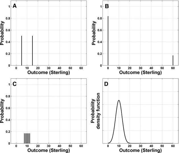
How can we quantify uncertainty? Imagine we could win £5 or £15 from heads or tails, respectively, at a coin flip, or £60 from a six on the dice and nothing for the numbers one to five. Are we more uncertain about how much we earn from the coin or from the dice? Figure 8.1a and b shows our expectations of winning the money from coin and dice. We do not have a deterministic expectation for either, so our expectations consist of a number of discrete probabilities. Panel c shows another case where we win the amount of money shown by the number on the dice, plus £6.50, and one can generalise this idea to situations with completely continuous outcome possibilities (panel d). What we have to find is a statistic that captures the amount of uncertainty embedded in each of these probability distributions. In the following, we give an overview of different statistics that are in widespread use, pointing out how they differ in their quantifications.


Fig. 8.1.
Probability distributions for four different gambles. a Flip of a fair coin with probabilities of 0.5 and a win of £5 or £15 from heads or tails, respectively. b Toss of a fair dice with a win of £60 from a six and nothing for the numbers one to five. c Tossing a fair dice again, winning the amount of money shown by the number on the dice, plus £6.50. d Probability density function for an unspecified example of continuous outcome possibilities.
Entropy (or Shannon entropy) is a measure from information theory (13) that is often used when outcomes are defined as a set of nominal and discrete events, one of which can occur at a time. Entropy takes only the probabilities for the occurrence of each event into account. That is, our uncertainty estimate does not depend on how much we win – it only depends on the probabilities of winning for each possible outcome. Entropy measures how much information we have about the upcoming event: we have some information about what will happen from throwing the dice, because we are not very likely to win. We have no information about the coin flip because both scenarios (head and tail) are equally likely. So, we should be more uncertain about the coin. That is reflected in entropy H, defined as the negative product of each probability with its (natural) logarithm, summed up over all possible outcomes:


For the three cases above, we derive
![$$\begin{array}{l}
H\left( A \right) = - \left[ {0.5 \cdot \log\left( {0.5} \right) + 0.5 \cdot \log\left( {0.5} \right)} \right] = 0.69 \\
H\left( B \right) = - \left[ {{\raise0.7ex\hbox{$1$} \mathord{\left/
{\vphantom {1 6}}\right.\kern-\nulldelimiterspace}
\lower0.7ex\hbox{$6$}} \cdot \log\left( {{\raise0.7ex\hbox{$1$} \mathord{\left/
{\vphantom {1 6}}\right.\kern-\nulldelimiterspace}
\lower0.7ex\hbox{$6$}}} \right) + {\raise0.7ex\hbox{$5$} \mathord{\left/
{\vphantom {5 6}}\right.\kern-\nulldelimiterspace}
\lower0.7ex\hbox{$6$}} \cdot \log\left( {{\raise0.7ex\hbox{$5$} \mathord{\left/
{\vphantom {5 6}}\right.\kern-\nulldelimiterspace}
\lower0.7ex\hbox{$6$}}} \right)} \right] = 0.45. \\
H(C) = \sum\limits_{i = 1}^6 {{\raise0.7ex\hbox{$1$} \mathord{\left/
{\vphantom {1 6}}\right.\kern-\nulldelimiterspace}
\lower0.7ex\hbox{$6$}}} \cdot \log {\raise0.7ex\hbox{$1$} \mathord{\left/
{\vphantom {1 6}}\right.\kern-\nulldelimiterspace}
\lower0.7ex\hbox{$6$}} = 1.79 \\
\end{array}$$](/wp-content/uploads/2016/07/A978-1-60761-883-6_8_Chapter_TeX2GIF_Equb.gif)
Thus, entropy prescribes in fact that we are more uncertain about the coin (A) than about the first dice throw (B) where we have two possible outcomes, one of which is much more likely than the other one. We are even much more uncertain about the outcome from the second roll of the dice (case C) where we have six possible outcomes, all with equal probability. However, it does not matter how much we earn, a perspective that economists and reinforcement learning theorists would probably disagree with. Does not the prospect of earning £5 or £15 from a coin flip feel much more uncertain than earning £9 or £11? The entropy is the same in both cases; however, their variance will differ.
Variance (and its square root, standard deviation) is an intuitive statistic that most researchers will be familiar with. It is commonly used to describe asset risk in finance (14) and hence has influenced behavioural economics and neuroeconomics where outcomes are defined in a continuous event space. Here, the magnitude of each possible outcome is taken into account. In the discrete case (A–C) variance is simply the squared deviation of each outcome from the expected (mean) outcome, weighted by the probability of this outcome and summed up over all outcomes (and similarly it can be generalised to continuous probability distributions as in case D). The expected earning in all three lotteries is £10, but the deviations from the mean are different. In case A, both possible outcomes (£5 and £15) deviate by £5 from the mean and have a probability of p i = 0.5, such that the variance (Note 1) is
 and analogous for the other two cases:


This time, we are most uncertain about B. This is because the earning from the six deviates so much from the average earning of the dice, and also from the earnings in the other two lotteries A and C. This conforms to our intuition about earning money, or goods: our earnings are more uncertain when the possible earnings have wider spread. Therefore, variance is a good statistic when values can be assigned to different outcomes (Note 2). If we change the earnings from the coin flip to £0 or £20, the variance increases to


However, adding a constant to both possibilities does not change the variance, which is possibly problematic. Earning £490 or £510 from a coin flip entails the same variance as earning £0 or £20. This might not seem very intuitive: many people would probably be more indifferent towards earning one of two amounts that are already quite large than towards earning either £20 or nothing. To reconcile this intuition with the idea of an uncertainty estimate, the coefficient of variation has been proposed (e.g. (15)) which is simply the standard deviation of outcomes, divided by the expected (average) outcome. This prescribes that we are more uncertain about our earnings when the same deviation occurs at a smaller average earning. In the example above, the coefficient of variation would be much smaller when the expected outcome is £500 than when it is £10.
We will see that entropy and variance (and its derivates) are the most commonly used measures of experimentally manipulated uncertainty in neuroscience. In some areas, proxy measures are being applied which we will discuss in detail below. All of these aim at quantifying the objective uncertainty given in the experimental situation. Of course it is possible that subjects have a different estimate of the uncertainty, for example, because they have prior assumptions which were generated outside the experimental context. An interesting question is therefore how one can quantify the uncertainty of actual neural representations. Naturally, prior knowledge and assumptions are usually beyond experimental control and can only be inferred from subjects’ behavioural or physiological responses. Therefore, we focus here on quantifying objective uncertainty but acknowledge that the actual uncertainty in neural representations might be slightly different.
4 Uncertainty About Sensory Information
4.1 Concepts
Sensory processing often involves categorising or quantifying incoming information. Uncertainty can then arise from noise in the sensory information or from uncertain representation of category templates, category boundaries or quantitative mappings. How can this be studied? Many experiments in this field are interested in how decisions are made when perceptual information is noisy and use decision-making models to describe the processes associated with the task. This will most often be some form of temporal integration model. We will therefore first give a brief overview of this class of decision-making models, then go on to show how measures from these models can be used as a proxy for the objective uncertainty.
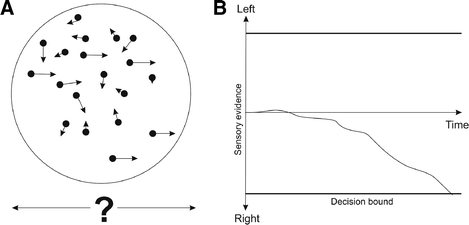
Temporal integration models (also termed sequential sampling, drift diffusion or bounded integrator models) assume that sensory information is accumulated over time (see for overviews, e.g. (17, 18)). Imagine, for example, an array of dots; 80% of dots are moving randomly to the right or to the left, the remaining 20% are consistently moving to the left (Fig. 8.2a). Our task is to decide whether the net movement is to the left or to the right. At each moment in time, the majority of dots could be – just by chance – moving to the right or to the left. Temporal integration models assume that we gather some evidence over time: at each moment in time, the number of dots we see moving to the right side causes a signal that is depicted in Fig. 8.2b. This could, for example, be a neuronal signal, achieved by summing up input from all neurons that detected a dot moving to the right, minus the signal from all neurons that detected a dot moving to the left. At each moment in time, the random dot motion causes this signal to fluctuate, but over time the consistent dot motion will cause the signal to increase (more or less) slowly. When this signal reaches a certain bound (criterion), we decide that the true movement direction is to the right. The opposite mechanism can account for a net movement to the left. The more random dots we add to this task, the shallower will the slope of this evidence curve be (the so-called drift rate), and the longer we will need to make a decision. At the same time, if we are forced to make a quick decision, we will be less accurate when there is more noise (18, 19).


Fig. 8.2.
Random dot motion task. a An array of dots is moving into random directions, with a proportion consistently moving left or right. The task is to detect the consistent motion direction. b Temporal integration model: Over time, evidence is accumulated for both possible motion directions; a decision is made when the evidence reaches a certain threshold.
Is there any place for uncertainty in this model? One might be tempted to use the drift rate as a surrogate for uncertainty, because the more uncertain the sensory evidence is, the smaller will the drift rate be. One can infer the drift rate from subjects’ behaviour: with a lower drift rate, reaction times would presumably be longer, and when there is an incentive for speedy responses, accuracy will be lower. However, the reverse relation is not necessarily given: shorter reaction times do not imply less certainty. In fact, reaction times can be biphasic such that people respond very quickly when there is little sensory evidence (20). Also, cerebral responses to reaction times and to accuracy dissociate although both should in theory depend on the drift rate (20); and cerebral responses to accuracy and objective task difficulty dissociate (21, 22). In addition, such temporal integration models have recently been challenged (16).
Beyond such measures for subjective uncertainty, there seem to be two principles of quantifying objective uncertainty in these tasks. A model-based approach to a categorisation task would measure the physical evidence for the different categories and quantify the uncertainty of the ensuing probability distribution over categories, for example, as entropy. On the other hand, one might measure physical similarity to a template or physical distance from a category boundary as a proxy for uncertainty. So far, most experimental paradigms use either accuracy or objective physical characteristics to quantify uncertainty. We will review three studies here that use these measures, but emphasise the need for a model-based approach in order to clearly define uncertainty.
4.2 Examples
4.2.1 Animal Experiments
Kepecs et al. (23) used an odour discrimination task in rats. Two pure odours (caproic acid and 1-hexanol) were mixed in six different ratios (0/100, 32/68, 44/56%). The rat’s task was to categorise the odour according to the major ingredient, with a reward for correct responses. Uncertainty was not quantified; instead the odour mixtures were treated as discrete levels: if the odour ratio was closer to 0.5, the perceptual uncertainty was assumed to be higher. The authors then investigated brain areas where neuron firing conformed to a U-shape or inverted U-shape when plotted according to the odour ratios, thus implying lower or higher firing with higher uncertainty. While this is a very elegant design, it shares a problem with most variations of perceptual uncertainty in reward-based decision-making. Because accuracy is lower with higher uncertainty, rats will learn to expect less reward with the intermediate odour categories. In order to disentangle neuronal responses to expected reward and to uncertainty, the authors performed a model-based analysis, comparing models based on either of the two factors.
Kiani and Shadlen (24) gave monkeys the random dot motion task described above, where the monkey had to make a saccade in order to indicate the net dot motion. Harvesting the fact that a more uncertain stimulus leads to a lower expected reward, they gave the monkey on half of the trials a chance to “opt out” and make a saccade to a third target which would yield a smaller, but fixed reward. Thus, they could measure the monkey’s estimate of his expected reward, corresponding to the confidence that his decision would be correct which can then be used as a behavioural measure of uncertainty in analysis of neuronal firing patterns. As in the example above, uncertainty is again correlated with expected reward, such that higher neural firing could be due to high uncertainty or low reward. Kiani and Shadlen avoid this confound by focusing on neurons that show either high or low firing when uncertainty is low, and intermediate firing when the uncertainty is high, and the monkey opts out. This corresponds to the temporal integration model shown in Fig. 8.1 where a fictive neuron that collects evidence for one motion direction would have high firing when the dots move into this direction, low firing when they move into the opposite direction and intermediate firing when the direction uncertain.
< div class='tao-gold-member'>
Only gold members can continue reading. Log In or Register to continue
Stay updated, free articles. Join our Telegram channel

Full access? Get Clinical Tree


