Principles of Angular Limb Deformity Correction

Introduction

Angular limb deformities (angular limb deformities) have long been a recognized source of lameness and debilitation in the small animal patient, and many articles have been written to guide the practicing surgeon toward accurate correction. We have begun an initiative to adapt a method of planning and correction commonly used in human surgery for the small animal patient. This method is called the center of rotation of angulation, or CORA, method. It was conceived by human pediatric orthopedic surgeon Dr. Dror Paley and was designed to achieve the following: (1) develop a system of angular limb deformity classification, (2) establish a vocabulary of terms to describe deformities and components of their characterization, (3) establish a library of reference ranges of “normal” bones to which the surgeon can refer, (4) propose a method of preoperative measurement that eliminates as much subjectivity and error as possible, and (5) provide guidance for accurate correction of angular limb deformities based on one standard set of geometric principles as they apply to osteotomies, regardless of the bone in question or the fixation device to be used.

The reader should recognize that because of the diverse and varied array of techniques described in the literature, this chapter is not an exhaustive review of all previously published work regarding the management of angular limb deformities. Rather, it is a synopsis of the CORA method of angular limb deformity correction, and it explains how the most relevant previously reported studies relate to knowledge of CORA techniques. Further, the methods presented herein primarily involve the treatment of dogs, because very little angular limb deformity research has focused on the cat. This is not to say that the principles reviewed here are not applicable to cats; however, a library of normal reference values has yet to be developed for the cat.

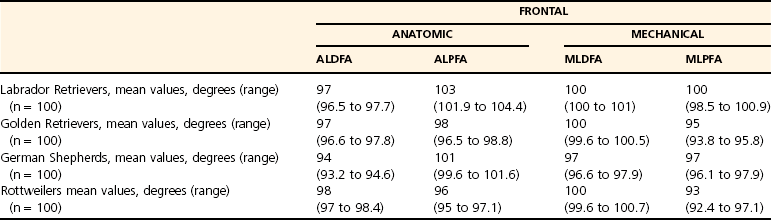
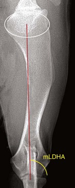
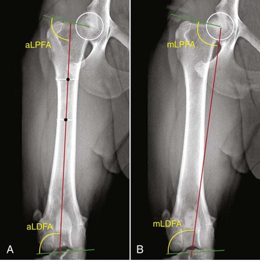
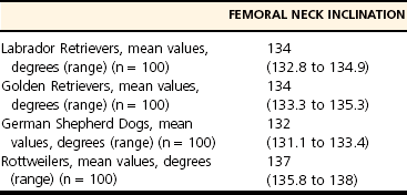
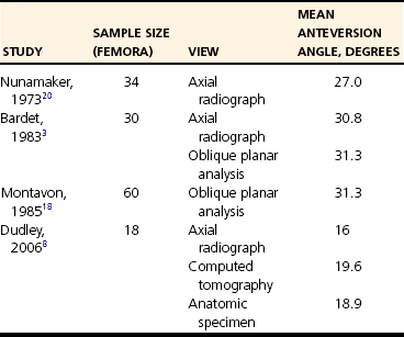
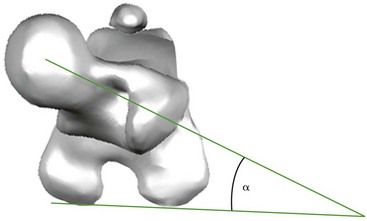
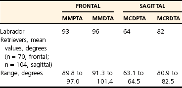
The research that supports this body of work is ongoing and continues to be refined and adapted for the small animal patient. Because of the breadth of the topic regarding angular limb deformity correction, this chapter should serve merely as a primer or introduction to the application of CORA principles. Angular limb deformity corrections are some of the most challenging orthopedic cases seen, and additional training should be sought before the techniques discussed here are attempted. The interested reader is encouraged to consult the text titled Principles of Deformity Correction, written by Dr. Dror Paley, because the principles discussed in this work are based on fundamental geometric concepts and thus are applicable to any bone or species.²¹

Normal Limb Alignment and Joint Orientation

The CORA method represents a system by which one can assess long bones for angular deformity. The technique requires that one understand the parameters of what is considered normal limb alignment. Bone alignment is objectively assessed through examination of bone axes, and joint orientation is evaluated using joint orientation lines. The intersection of an axis and a joint orientation line forms a joint orientation angle that defines the relationship of the joint to the rest of the bone. The bone axes (anatomic and mechanical), joint orientation lines, and joint orientation angles constitute the basic building blocks for determining what is “normal,” so that affected bones can be assessed objectively.

Defining Frontal, Sagittal, and Transverse Planes

Deformities can occur in one of three planes: frontal, sagittal, or transverse. A plane is defined as a flat surface, the position of which is determined by three points in space. Radiographic images are used to assess planes. The frontal plane is examined from a cranial-to-caudal radiographic image and is used to evaluate for valgus or varus deformity (lateral or medial deviation, respectively). The sagittal plane is assessed from a lateral-to-medial radiographic image and is used to evaluate for procurvatum (cranial bowing) and recurvatum (caudal bowing). The transverse plane is studied from an image obtained with the beam directed axially along the bone and is used to evaluate for torsional deformity. Some bones have deformities in more than one plane. Six possible deformational directions have been noted. By convention, a deformity is described in terms of the relationship of the distal portion of the bone or joint to the more proximal portion of the same structure.

Bone Axes

Standardized methods are important in assessing each bone. The method used should remain consistent, regardless of bone or observer. Bones are evaluated in both frontal and sagittal planes; however, additional radiographic views can be obtained if needed. The first tool for assessing a bone consists of determination of bone axes. Axes are defined as anatomic or mechanical and can be established for an entire limb or for a specific bone.⁶ This chapter focuses on evaluation of individual bones. The anatomic axis is defined as a line that passes though the center, or mid-diaphysis, of the bone in the frontal or sagittal plane. Because the anatomic axis follows the geometry of the bone, if the bone is very straight, only one line will be centered between the two cortices. An example of this situation is seen in the canine radius in the frontal plane (Figure 47-1, A). In situations involving natural curvature, the anatomic axis will also be curved. However, the curved anatomic axis can be resolved into multiple straight segments to allow quantification of the angulation of curvature. Thus, when the radial anatomic axis in the sagittal plane is assessed, the procurvatum of the anatomic axis can be expressed as two straight lines (Figure 47-1, B).

Figure 47-1 Joint orientation lines (green) and anatomic axes (red) of the canine radius in frontal (A) and sagittal (B) planes from which the joint orientation angles (yellow) are calculated. aCdDRA, Anatomic caudal distal radial angle; aCdPRA, anatomic caudal proximal radial angle; aLDRA, anatomic lateral distal radial angle; aMPRA, anatomic medial proximal radial angle. Note that in the sagittal plane, two anatomic axes are used to resolve the natural procurvatum of the radius; the difference between the axes is quantified as θ.

Given the sigmoidal shape of the canine tibia in the frontal plane, the anatomic axis is established by identifying multiple straight components. For bones such as this, identification of a mechanical axis has greater clinical usefulness. The mechanical axis is defined as the straight line connecting the center points of the joints proximal and distal to the bone in the frontal or sagittal plane (Figure 47-2). The mechanical axis is always a straight line and represents the weight-bearing axis of the bone. Clinically, the anatomic axis is most easily used to assess bones that are normally straight in a particular plane (e.g., the canine radius in the frontal plane), and the mechanical axis is most easily used to define a bone that is normally curved (e.g., the canine tibia in the frontal plane).

Figure 47-2 Joint orientation lines (green) and mechanical axis (red) of the canine humerus in the frontal plane from which the joint orientation angles (yellow) are calculated. mLDHA, Mechanical lateral distal humeral angle. The center of the shoulder joint is estimated from a best-fit oval superimposed over the humeral head (white).

A joint orientation line represents the orientation of a joint in a particular plane. This line is determined by selecting two bone-specific anatomic landmarks on each joint surface that are repeatable from bone to bone in a specific plane. The intersection of the bone axis and the joint orientation lines results in quantifiable joint orientation angles that define the relationship between the surface of the joint and the particular axis used (see Figure 47-2). The joint orientation angles are named for the axes, joint orientation lines, and bone sidedness that characterize them and are always named in the same sequence. A small letter “a” or “m” is used to designate whether the angle was derived from the anatomic or mechanical axis. The next capital letter designates whether the angle is measured on the cranial (Cr) or caudal (Cd) side if the sagittal plane is being assessed, or on the medial (M) or lateral side (L) if the frontal plane is being assessed. The next capital letter signifies whether the measurement is of the proximal (P) or distal (D) end of the bone. Next, a letter representing the bone measured is listed (e.g., “F” is used for femur, “R” for radius). Finally, a capital “A” is used to stand for the word “angle.” Thus, the designation aLDFA means that the anatomic lateral distal femoral angle was measured, whereas mMPTA would represent the mechanical medial proximal tibial angle. A list of the joint orientation angles that have been derived for specific bones in specific planes for each major long bone are presented here. These reference values are invaluable when a bilaterally affected patient is presented for correction, thus offering no contralateral side for comparison. To date, not all bones have been fully assessed and differences between breeds are still incompletely understood, although breed differences are likely, given the findings of ongoing studies. A brief overview of the axes and joint orientation lines and angles for the major long bones is provided in the following sections.

Humerus

Little information is available regarding assessment of deformity of the canine humerus. One study defined a method of determining the bone axis and joint orientation line, and reported values for the distal joint orientation angles in the frontal plane.²⁷ Craniocaudal radiographs were obtained by ensuring that the elbow joint was straight and perpendicular to the x-ray beam. A frontal plane “elbow straight” radiograph is defined by (1) no appearance of the medial or lateral surfaces of the anconeal process, and (2) distance from the medial epicondyle to the medial cortex of the olecranon equivalent to 45% of the transcondylar distance.⁹

To determine the humeral mechanical axis, a best-fit oval is centered over the humeral head, and the center of the oval is determined. At the distal end of the humerus, a joint orientation line is drawn from the distalolateral-most aspect to the distomedial-most aspect of the humeral condyle. The midpoint of this line is determined. The mechanical axis is drawn from the center of the humeral head to the center of the humeral condyle (see Figure 47-2), and the mechanical lateral distal humeral angle (mLDHA) is measured. The mean value reported for the mLDHA was 87.3 ± 2.9 degrees for a population of large-breed, nonchondrodystrophic, skeletally mature dogs.²⁷

Radius

Because the radius is the predominant weight-bearing bone of the antebrachium, and because it provides the largest articular surface for both the elbow joint and the carpal joint, it is the bone that receives the greatest focus regarding assessment for angular correction. Methods used for its evaluation have been described.9,11 Radiographic positioning can utilize the aforementioned elbow straight criteria in the frontal plane to eliminate the effect of antebrachial torsion on joint orientation line measurement. The landmarks that determine the proximal radial joint orientation line in the frontal plane are the proximolateral edge of the radial head and the medial portion of the coronoid process. If these points are obscured or affected by osteophytes, the distal aspect of the humeral condyle (as described for the humerus) can also be used, as long as no soft tissue laxity is present within the joint. For the distal radial joint orientation line, reference points include the lateral-most aspect of the articular surface and the medial aspect of the articular face, ignoring the styloid process. The anatomic axis is drawn by connecting three points with a best-fit line that bisects the radius at levels within the metaphyses and mid-diaphysis. The angles that are measured for the proximal and distal ends of the radius are the anatomic medial proximal radial angle (aMPRA) and the anatomic lateral distal radial angle (aLDRA), respectively (see Figure 47-1, A).

In the sagittal plane, radiographic repeatability is ensured by centering the elbow so that two concentric circles can be superimposed over the medial and lateral aspects of the humeral condyle, and these circles do not intersect.⁹ The reference points for the proximal radial joint orientation line are the most proximal extent of the cranial and caudal aspects of the radial head. The reference points for the distal radius are the cranial and caudal aspects of the radial articular surface. Note that the radius has a normal procurvatum. As a result, the anatomic axis in the sagittal plane is curved but may be resolved into two segments—one for the proximal half of the bone and one for the distal half of the bone. To determine the two anatomic axes, two points are found that bisect the radius in the proximal and distal halves of the diaphysis. The respective reference points are connected in both halves of the bone to form the two anatomic axes whose intersection (θ) is within the cortical confines of the bone and is quantifiable (see Figure 47-1, B). The anatomic caudal proximal radial angle (aCdPRA) and the anatomic caudal distal radial angle (aCdDRA) are measured (see Figure 47-1, B). Because the natural procurvatum of the radius exists along the entire length of the bone, calculating it requires summation of the proximal and distal joint orientation angles and of the difference between segmental anatomic axes (θ). Thus the formula (90 degrees − aCdPRA) + (90 degrees − aCdDRA) + θ yields overall procurvatum in degrees.⁹ Reference values for the joint orientation angles and the procurvatum are presented in Table 47-1.

Table • 47-1

Mean Radius Joint Orientation and Procurvatum Angles As Measured in 100 Labrador Retrievers ⁹

aCdDRA, Anatomic caudal distal radial angle; aCdPRA, anatomic caudal proximal radial angle; aLDRA, anatomic lateral distal radial angle; aMPRA, anatomic medial proximal radial angle.

Femur

A standardized method of evaluating the canine femur in the frontal plane has been described.³¹ Similar to the other bones, the femur must be positioned in a true craniocaudal orientation and parallel to the table top if it is to be accurately measured. Characteristics of a well-positioned femur include the appearance of the walls of the intercondylar notch, with the fabella appearing to be bisected by respective femoral cortices and the slight protrusion of the corticocancellous tip of the lesser trochanter.¹⁵ Although some studies have shown that femoral parameters can be measured accurately with radiographs when compared with anatomic specimens, others have shown that radiographic measurements may not be true predictors of the degree of angulation, specifically when distal varus is considered.³⁰ Because radiography remains the most commonly used tool to assess canine long bones, a standard method by which to assess the axes and joint orientation lines as a reference for what can be considered normal is required. The distal joint orientation line is determined by a line that just touches the distal-most aspect of the lateral and medial femoral condyles (Figure 47-3). The proximal joint orientation line runs from the center of the femoral head to the dorsal-most aspect of the greater trochanter of the femur. The anatomic axis is determined by a line that connects points selected 33% and 50% below the proximal aspect of the femoral neck in the middle of the femur (Figure 47-3, A). One will note that distally, the anatomic axis deviates from the center of the bone. Whereas the anatomic axis of the femur should actually be drawn to slightly curve medially, reflecting a normal distal femoral varus, Tomlinson and associates instead document how if the axis is kept straight, it frequently passes just lateral to the intercondylar notch.³¹ The anatomic lateral distal femoral angle (aLDFA) is measured as the intersecting angle of the anatomic axis and the distal femoral joint orientation line. The anatomic lateral proximal femoral angle (aLPFA) is measured as the angle that is formed by the anatomic axis and the proximal femoral joint reference line. The mechanical axis is determined by a line that runs from the center of the femoral head to the center of the distal femoral joint orientation line (Figure 47-3, B). The mechanical lateral distal femoral angle (mLDFA) is measured as the angle that is formed by the mechanical axis and the distal femoral joint orientation line. The mechanical lateral proximal femoral angle (mLPFA) is measured as the angle that is formed by the mechanical axis and the proximal femoral joint reference line. Normal angles vary by breed; measured angles for four breeds of dogs are listed in Table 47-2.

Table • 47-2

Mean Femoral Orientation Angles in the Frontal Plane for Both Anatomic and Mechanical Axes ³¹

aLDFA, Anatomic lateral distal femoral angle; aLPFA, anatomic lateral proximal femoral angle; mLDFA, mechanical lateral distal femoral angle; mLPFA, mechanical lateral proximal femoral angle.

Figure 47-3 Anatomic (A) and mechanical (B) axes (red) of the canine femur in the frontal plane with associated joint orientation lines (green) from which the joint orientation angles (yellow) are calculated. aLDFA, Anatomic lateral distal femoral angle; aLPFA, anatomic lateral proximal femoral angle; mLDFA, mechanical lateral distal femoral angle; mLPFA, mechanical lateral proximal femoral angle. The center of the femoral head is estimated from a superimposed best-fit circle (white).

The angle of inclination and the anteversion angle of the femur are two parameters that are frequently measured when the femur is assessed. The inclination angle of the femoral head and neck is measured from the frontal plane radiograph and is the angle formed by the proximal femoral anatomic axis and a line that originates at the center of the femoral head and bisects the femoral neck.13,31 Coxa vara is defined as a decreased angle of inclination, and coxa valga as an increased angle of inclination.^12,26 Figures for normal femoral neck inclination vary depending on the study and the breed, but values collected for a large case series of four different breeds are presented in Table 47-3.

Table • 47-3

Femoral Inclination Angles in Four Breeds of Dog ³¹

The anteversion angle of the femoral head and neck is defined as the angle between the neck and the frontal plane, as described by the caudal aspect of the femoral condyles (Figure 47-4). The anteversion angle can be determined with the use of computed tomography (CT) or axial radiography, or it can be calculated by oblique planar analysis using graphical or trigonometric methods. For axial radiography, the image is obtained with the femur in a vertical position, so that the femoral head and neck and the distal aspect of the femoral condyles are visible and superimposed. A line is drawn from the center of the femoral head to a point that bisects the femoral neck. A second line is drawn so that it just touches the caudal aspect of the femoral condyles.²⁰ The angle formed by the intersection of these two lines is the anteversion angle (see Figure 47-4). Whereas this technique results in version angles comparable with those achieved with CT, the view can be challenging to obtain and frequently requires fluoroscopy to aid with satisfactory positioning.⁸ Standard orthogonal radiographs can also be used to calculate the version angle by way of oblique planar analysis.^3,18 Normal anteversion angles vary widely between studies (Table 47-4).

Table • 47-4

Femoral Anteversion Angles As Reported in Four Studies

Figure 47-4 Schematic of the axial view of the canine femur demonstrating the positioning necessary to achieve the radiographic calculation of femoral anteversion (α), which is the angular difference between a line drawn across the caudal-most aspect of the femoral condyles and a line bisecting the femoral head and neck.

Tibia

When the tibia is radiographed in the frontal plane, the criteria described for the distal femur can be used to ensure “knee straight” radiographs, which also allow straight positioning of the proximal tibia if no stifle joint subluxation is present. In the sagittal plane, the medial and lateral condyles of the tibial plateau should be superimposed. A standardized method used to measure the tibial joint surface angles, in relation to the mechanical axis, in the frontal and sagittal plane has been described.4,5 In the frontal plane, the most distal points of the subchondral bone concavities of the medial and lateral tibial condyles are used as landmarks for the proximal tibial joint orientation line (Figure 47-5, A). The most proximal points of the subchondral bone of the two arciform grooves of the cochlear tibiae are used as landmarks for the distal tibial joint orientation line. A mechanical axis is used because of the natural sigmoidal shape of the tibia in the frontal plane. The mechanical axis of the tibia is defined by a point in the center of the proximal-most aspect of the intercondylar fossa of the femur and at the most distal point of the subchondral bone of the distal intermediate tibial ridge (see Figure 47-5, A). Because the tibial plateau is sloped in dogs, a tangential view of the proximal tibia may more accurately quantify frontal plane angulation arising from this portion of the bone.¹⁶ The angles between the mechanical axis and the joint orientation lines are measured on the proximomedial and distomedial aspects to determine the mMPTA (mechanical medial proximal tibial angle) and the mMDTA (mechanical medial distal tibial angle), respectively. Reference values for mMPTA and mMDTA are provided in Table 47-5.

Table • 47-5

Mean Tibia Joint Orientation Angles As Measured in Labrador Retrievers 4,5