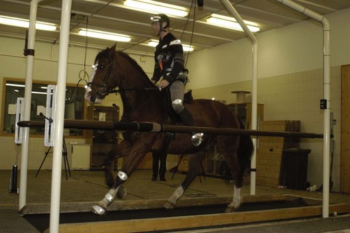
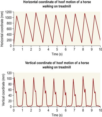
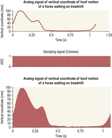
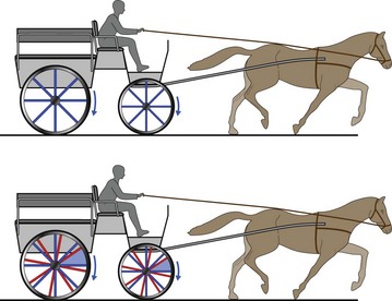
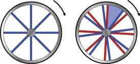
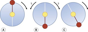
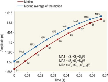
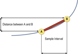
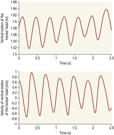
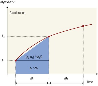
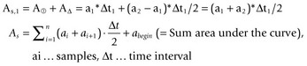
Chapter 3 In equine motion analysis a signal is a measured physical property of a movement presented as time-depended parameter or variable. It is acquired by different measurement methods, such as kinematic measurement (Fig. 3.1). This physical parameter can be a coordinate (distance from origin), a force, acceleration, an angle and so on. These signals are so-called bio signals. A bio signal presents a time series of a physical parameter of a living being (Shiavi, 1999), and appears naturally in time-continuous form. Figure 3.2 presents a typical signal in time-continuous form. Due to the measuring technique (analog to digital converter (ADC)) today nearly every signal is detected as digital signal (Semmlow, 2004). The ADCs quantify the captured values. The effective range is always a power of 2. So a 12-bit ADC means that the effective range is divided into 212 (4096) steps. A digital signal consists of values measured at given time points, in most cases time-equidistance. Figure 3.3 shows the sampling (measuring) process of a signal. Normally noise and/or any other disturbances interfere with the desired signal (Semmlow, 2004). Sources of these disturbances may be errors of the measurement equipment, ADC (quantization error), influence of an electrical field in case of EMG or ECG, etc. DSP is necessary to get the most out of the measured data. The first step is to set up the measurement equipment in a way that the digital signal represents the measured signal sufficiently. Certain preconditions have to be fulfilled to represent a time continuous signal by a digital signal (time-equidistance sampled values). This characteristic is described by the Nyquist – Shannon sample theorem (Oppenheim & Willsky, 1996; Semmlow, 2004). The last graph of Figure 3.3 shows a sampled signal. Now the question arises, is the sample frequency sufficient? In movies there is often a strange effect in moving stagecoaches. It is clearly visible that the stagecoach moves from left to right. But the wheels of the stagecoach appear to be revolving in the opposite direction (Figs 3.4 and 3.5). Figure 3.6 shows another example of a turning wheel with more spokes. The conclusion is that in fast movements more than 16 pictures/turn (because there are eight segments) are necessary. The conclusion of the wheel experiment is the Nyquist – Shannon sampling theorem, which states that the sampling frequency must be at least twice the signal frequency to avoid the alias effect (Werner, 2006): Normally oversampling is used during the measurement. For instance, a sampling frequency that is five times higher than the theoretical minimum sample frequency is used. Often two different measurement systems are synchronized, e.g. a kinematic system with a force plate or EMG equipment. Both systems use different sampling frequencies. Since EMG measurements need a much higher sampling frequency than the kinematic measurements, the result is two different time scales, i.e. one for kinematic and one for EMG. To solve this problem, resampling is needed. If the sample frequency from EMG is reduced (Peham et al., 2001a,b; Licka et al., 2004), it is comparable to smoothing or low-pass filtering. If there is a whole-numbered relation between the two sample frequencies, it is very easy to reduce or add the samples. The simplest method to reduce the samples is for instance to take only every second or third sample and to add samples to calculate the values of the new samples by a linear relation between two neighboring samples. Usually the procedure of resampling is done in two steps. The first step is to fit the curve (e.g. cubic spline, Fourier series, etc.) in the second step; the new samples will be extracted from the fitted curve. If the sample frequency is to be reduced, it is necessary to limit the bandwith by a low-pass filter. In case of a moving average of three, the mean is calculated from the first three samples ( (s1 + s2 + s3)/3) to give the first new sample. The next sample will be calculated by the mean of the samples shifted by one ( (s2 + s3 + s4)/3) and so on (Fig. 3.7). This is a kind of resampling with the reduction of the sampling frequency. The effect is a shift of the curve by one sample interval. If a moving average of five samples is used, the delay will be two sample intervals and so on. This combination of more samples is very similar to a reduction of the sample frequency. So if it is used, it must be realized that the signal is now low-pass filtered. A resampling is also evident when the duration of a motion cycle is normalized to 100%. Normalization or a relative time scale is used as it makes the comparison of different motion cycles easier, and allows averaging of multiple movement cycles into a single curve (a so-called ‘ensemble average’). The disadvantage is that the absolute time scale is lost. Sometimes the information of the variation of the duration of motion cycle is needed, which is then done before normalization. Figure 3.7 shows a signal and the smoothed signal with a moving average of three samples. It is obvious that the smoothing will shift the signal. Figure 3.8 shows one sample interval of a coordinate motion. The sample rate gives us the time scale, whereas the coordinates give the distance from A to B. The velocity for each sample interval is calculated by dividing the distance between two samples by the duration of a sample interval. The mean velocity for each interval is the quotient of the distance and the elapsed time. The motion is represented by the slope of a straight line between two points. If the sample rate is infinitive, the straight line is the tangent to this curve at a given time point. In the real world the sample rate is always finite. So in DSP it is possible to calculate the mean velocity between two consecutive measures. Time series of velocity can be calculated by repeating this step for all intervals. Phase-plane analyses are used to show the stability of a system or a motion. Examples are stability of equine gait on a treadmill (Peham et al., 1998), harmony of horse and rider (Peham et al., 2001c) and stability of coupling via saddle of horse and rider (Peham et al., 2004). A phase-plane is a graph of a signal (motion) versus its derivative (speed). Figure 3.9 shows the motion (first graph) and the velocity (second graph) of vertical motion of the head of the horse. Since the differentiation is the local linearization, the curve can be replaced by tangents in every time point. We presented here only the simple linear method of differentiation (Fig. 3.8). More point methods (e.g. 5-point) based on the Taylor series are often used. When differentiation is applied to data that contains noise, results can be inaccurate. This will be discussed later. In Figure 3.9, it can be seen that when the head goes up the velocity is positive. When the head goes down the velocity is negative. Integration is very important in motion analysis. Additionally, many powerful mathematical tools are based on integration, e.g. differential equations are the direct consequence of the development of integration. Calculation of impulse from the time curve of force (Osterlinck et al., 2009), integrated EMG (Wijnberg et al., 2009), and computation of speed from acceleration (Galloux et al., 1994) are a few examples of integration in motion analysis. Figure 3.10 shows how the area under a curve can be calculated. The first step is computation of area of the square (side length = first sampled acceleration a1, Δt1 = sample interval) A1 = a1 × Δt1. The rest of the area is a right-angled triangle (side length a = difference between the first and the second sampled acceleration a2 − a1, side length b, Δt1 = sample interval) A2 = (a2 − a1) × Δt1/2. The equation above shows the calculation of the area for one interval and then for n sampled values (n-1 intervals).
Signals from materials
Introduction and definition of signals
Choosing the sampling frequency (Nyquist – Shannon sample theorem)
Motion of a wheel

Resampling and normalization
Signal processing
Time curve analysis
Differentiation
The physical concept of Newton
Phase-plane analysis (practical use of differentiation)
Increasing, decreasing and finding a local maximum or the minimum (extreme values)
Integration
Signals from materials