History of computer modeling

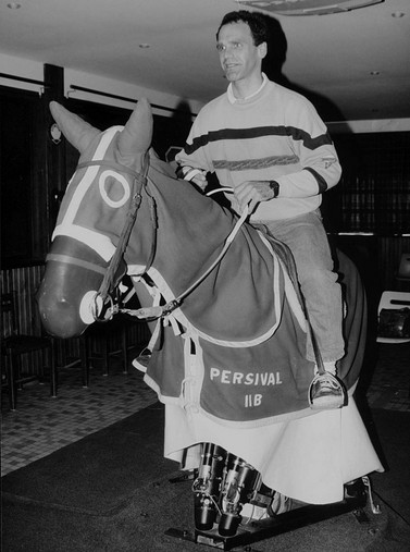
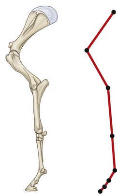
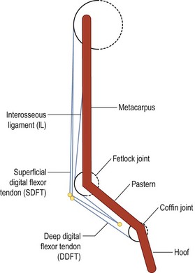
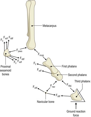
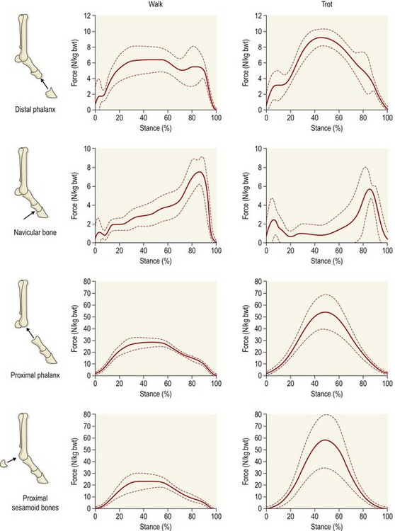
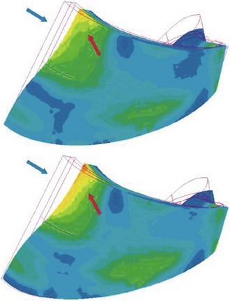
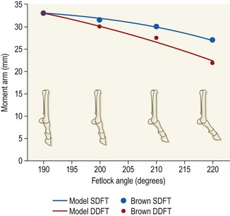
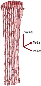
The origins of computer modeling can be traced back to a program developed in 1963 at the Massachusetts Institute of Technology (Encarnacao et al., 1990). Its capabilities were limited to what would be called a simple drawing program in modern terms, but many of the fundamental drawing subroutines and standards were established by this work. Although developments were made in subsequent years, it wasn’t until the late 1970s that computer-based design moved from the realm of academic theory into mainstream science. As the increasing power of computers allowed for more advanced applications, a new technique was developed in the 1980s called ‘solid modeling.’ In this process a three-dimensional representation of a structure is created within a computer, rather than the older method of simply having a number of two-dimensional projections.

Using this new technology, designers could view parts of a system and their interactions without the cost and time involved in creating a prototype. Assemblies of independent components, structural supports, or even entire complex mechanisms such as automotive engines could be examined for fit and accuracy before any real monetary investment was made by the company.

Applications of computer models

There are four typical applications of computer models in biomechanics: visualization, kinematics, dynamics and finite element analysis.

Visualization

The potential of computer models in visualization represents one of the great emerging applications of this technology. A well-known example is the use of CT or MRI data by a veterinarian or physician to produce a three-dimensional recreation of a bone or joint, rather than looking at it as a series of two-dimensional projections. This functionality is included in a number of commercial medical imaging products. The operator uses specific areas as ‘edges’ of structures and the computer rebuilds a visualization of the bone, soft tissue or any other object of interest. This type of modeling is useful for viewing different structures and the relationships between them in live subjects, but some of its most promising practical applications arise from the ability to produce physical objects by the processes of rapid prototyping and machining.

Rapid prototyping is a method by which a sample part is made from (typically) a soft plastic or other suitable material that can be held and examined, not just viewed on a computer screen. The process consists of creating a solid model in the computer, then sending the information to a rapid prototyping machine, which recreates it as a series of layers of the material. In industry, entire prototype engines have been constructed this way to demonstrate new technology and concepts that would be difficult to otherwise describe. Similarly, anatomical structures can be recreated and examined in the same way as a dissected specimen. This has been explored in humans as a method of preparing surgeons to perform operations, including neurological and orthopedic procedures (McGurk et al., 1997).

Machining is a process by which a product is manufactured from a permanent material. For orthopedic procedures, this allows preliminary evaluation of surgeries and the manufacturing of custom implants. Using CT data obtained preoperatively, the joint can be recreated precisely in the computer and a surgeon can have an exact fit for the orthopedic implant prepared prior to surgery or even constructed during the procedure (Mulier et al., 1989).

One of the most exciting areas into which visualization techniques are expanding is the field of virtual reality. The concept of virtual reality has become something of a buzzword of the media in recent years due to proliferation of home computers, increased distance interaction on the internet, and incredible advances in computer graphics. The true concept of virtual reality is that, by recreating a situation in the processor of a computer and by using highly realistic graphics, the human brain can be fooled into believing that the computer-generated images are real. Although technological limitations still prevent complete immersion in a virtual reality environment, some early demonstrations of its medical applications have been performed, such as the National Library of Medicine’s Visible Human Project. This is an ambitious program to develop a complete database of human anatomy based on cryosections and CT scans of male and female cadaver specimens. The results of this research have already been used to develop educational and research tools for audiences ranging from school-age children to medical professionals.

Another focus for the development for visualization tools in medicine is in preoperative planning. An entire surgery can be simulated and performed any number of times to rehearse the mechanics of the procedure prior to a single incision being made on a live patient. However, the use of a purely anatomical model cannot completely prepare the student for all situations and complications that may arise during a procedure and that necessitate a rapid and accurate response by the surgeon. However, in the same way that pilots can practice emergency maneuvers and landings in jet simulators, critical conditions could be simulated to prepare a student for surgical emergencies.

The application of virtual reality in the field of equine biomechanics is quite advanced. An early example is ‘Persival,’ a mechanical horse simulator (Fig. 20.1) developed by Patrick Galloux of the Ecole Nationale d’Equitation in Saumur, France (Galloux et al., 1994). His group has constructed a mechanical simulator that recreates the movements of a horse at a walk, trot and canter, as well as during jumping. Virtual reality is used to allow the rider to follow a show jumping course by watching a screen in front of the simulator or by wearing virtual reality glasses. The rider sees the obstacles, and sensors are used to detect and react to the rider’s aids. It has been found that by using this simulator, the time required to train a rider was shorter than when using a real horse, and the novice rider was able to learn safely and without the need for ‘lesson’ horses. A horse simulator is also available that allows the ride to experience and replay a virtual dressage test (http://www.racewood.com/dressage.php).

Kinematics (movement)

Kinematics is defined as the observation of motion in a mechanical system. It encompasses a spectrum that ranges from the rotation of a horse’s limbs as it gallops across a polo field, to the movements of a player’s arm and mallet as a shot is made, to the way the polo ball arcs through the air after it has been hit. Kinematic studies have described the horse’s movement at various gaits and during jumping. This information can be used to create an accurate simulation of the motion of a particular joint that shows how the various components interact and allows the user to visualize the effects of disease, lameness or surgeries. Other types of computer simulations might show deformation of the structures within the hoof during weight bearing, or the actions of the rider in giving a horse the aids for different movements.

It is important to recognize that kinematics is limited to the process of observation; it does not have the ability to make inferences. For example, kinematics can be used to study how a bone, joint, limb or animal moves based on a set of data describing that movement, but it cannot predict the results of a perturbation of the system, such as an injury or lameness. Using computer models as kinematic simulations is, to a great extent, a specific application of the previously discussed visualization tools. However, it goes beyond simple visualization because the kinematic information represents a bridge between visualization, a purely external observation, and dynamics, an understanding of the forces that are responsible for creating the movement and the forces that arise as a consequence of the movement. Halvorsen et al. (2008) used filtering for optimally tracking kinematics. Bobbert & Santamaría (2005) and Bobbert et al. (2007) used body kinematics to calculate limb dynamics (Bobbert et al., 2007) and energetics (Bobbert & Santamaria, 2005).

Kinetics (dynamics)

As stated above, kinematics is a passive observation of how a system moves. Dynamics uses kinematic data, combined with additional information, to evaluate the forces within the system. Having calculated the dynamics, much more complex simulations can be performed. Two methods are primarily used for the development of dynamic results: inverse dynamics, and forward or direct dynamics. In general, inverse dynamics is a technique by which internal forces are estimated using data from external observations, while forward dynamics predicts external forces and motions by prescribing internal forces. An application of computer modeling using inverse dynamics involves the calculation of net joint moments and joint powers from knowledge of the kinematics, ground reaction forces (GRFs) and morphological data using a link-segment model. In this type of model, the complex structure of the limbs is simplified by representing the limb segments as rigid bodies linked by hinge joints (Schryver et al., 1978; Hjertén & Drevemo, 1987; Clayton et al., 1998; Colborne et al., 1998; Lanovaz et al., 1999) (Fig. 20.2). The musculature that drives the limb has a complex geometry and many mechanical and material properties that are difficult to quantify. In order to study the effect of muscle action without defining all of the specific parameters of the system, the net muscular action within the limb is represented in the model as net torques or net joint moments acting at each of the joints. Zarucco et al. (2003) developed and tested an experimental model for in-vivo short-term recording of peak isometric forces of the digital flexor muscles in the forelimb of adult horses and thus provided further insight to functional implications of the complex architecture of these muscles. Realistic inertial parameters such as mass and moment of inertia are assigned to each segment of the computer model. Kinematic data and GRFs are measured and used as inputs to the model. An inverse dynamics solution is used to calculate the torques required to cause the observed motion and forces. This ‘net effect’ of muscle action derived from the model can be applied in both clinical and research settings to study the function and dysfunction of the limb at the different joints (Buchner et al., 1996; Clayton et al., 1998). Brown et al. (2003) developed a detailed musculoskeletal model of the distal equine forelimb to study the influence of musculoskeletal geometry (i.e. muscle paths) and muscle physiology (i.e. force–length properties) on the force- and moment-generating capacities of muscles crossing the carpal and metacarpophalangeal joints. They predicted that the suspensory and check ligaments contributed more than half of the total support moment developed about the MCP joint in the model. Additional information can be added to the model to increase the level of sophistication. For example, knowledge of the orientation of anatomic structures such as the line of action of tendons can allow for a more detailed estimation of internal muscle and tendon forces (Riemersma et al., 1988; Jansen et al., 1993). Merritt et al. (2008) developed a two-dimensional model of the musculoskeletal system of the distal limb region and applied it to kinematic and kinetic data from walking and trotting horses. The forces in major tendons and joint reaction forces were calculated. The components of the joint reaction forces caused by wrapping of tendons around sesamoid bones were found to be of similar magnitude to the reaction forces between the long bones at each joint. This finding highlighted the importance of taking into account muscle-tendon wrapping when evaluating joint loading in the equine distal forelimb (Figs 20.3–20.6).

Swanstrom et al. (2005) developed a musculoskeletal model of the Thoroughbred forelimb and a dynamic simulation of the motion of the distal segments during the stance phase of high-speed (18 m/s) gallop. The musculoskeletal model was comprised of segment, joint, muscle-tendon, and ligament information. The dynamic simulation incorporated a proximal forward-driving force, a distal ground reaction force model, muscle activations, and initial positions and velocities. A simulation of the gallop after transection of an accessory ligament demonstrated increased soft tissue strains in the remaining support structures of the distal forelimb, consistent with those previously reported from in vitro studies. Forward or direct dynamics utilizes data describing muscle activation patterns and the force of muscular contraction to determine the position of each segment of the limb. Although this method is theoretically ideal, as it is the most accurate representation of what is actually occurring in the system, it is practically difficult to measure these inputs with the accuracy needed to produce a model that represents the internal forces and interactions. A variation on this type of dynamic analysis was performed for an entire horse in 1987 using a mechanical mechanism analysis package (Van den Bogert, 1989). The horse was represented by a series of rigid bodies connected by springs, dampers and torque producers representing tendons and ligaments. The innovative aspect of this simulation was that, instead of simply prescribing the motion of a segment by kinematic data, an intelligent model was created that prescribed the limitations of joints, the reaction forces created by the tension in ligaments and muscle activations. The model was analyzed and validated through both kinematic and ground reaction force data. However, in order to simulate the entire horse, a number of assumptions had to be made due to the complexity of the project and the limitations in computer power at the time. The entire system was assumed to be purely two dimensional with the segments of the horse moving in the sagittal plane. Complex joints, such as the carpus and tarsus, were approximated as simple hinges, and it was necessary to completely ignore certain joints, such as the coffin joint and the articulation of the spine. In spite of these assumptions, the simulation was found to accurately recreate the ground reaction force patterns measured in research studies.

Musculoskeletal models have been used to investigate underlying concepts of equine locomotion that are often broadly accepted, but not understood in detail. Merritt et al. (2010) investigated the function of the fetlock joint and found that the metacarpus was loaded in compression by the combined actions of the proximal sesamoid bones and the first phalanx. Although this kind of compressive loading was already understood to exist in the metacarpus, the study illustrated the extent to which this loading depended upon the concerted function of the entire forelimb, rather than being a feature of the fetlock alone. Harrison et al. (2010) utilized an extensive forelimb model to investigate elastic energy storage and release in the distal forelimb. Elastic energy storage had long been considered an important feature of locomotion in large animals, but these authors were able to quantify its role in detail for the first time. Even in the muscular structures of the distal forelimb, such as the superficial and deep digital flexor muscles, these authors reported that between 69–90% of the total work was done by elastic energy release, rather than by active muscle contraction, with the amount of elastic energy storage increasing at faster speeds. Studies of this kind help to close critically important gaps in overall understanding, by providing the detailed mechanisms of action for features of locomotion, which were previously understood in only the broadest terms.

The availability of a complete and accurate model of even a single joint opens up incredible opportunities. Should a specific treatment be recommended, such as a tenectomy, the outcome can be predicted by incorporating into the model the loss of the forces transmitted by that tendon. The model could then be used to predict the effectiveness of the treatment, allowing for a more educated and confident recommendation of the likely benefits. This application was validated by a study in which the human lower leg was recreated in a computer to evaluate orthopedic surgical procedures. It was found that the model accurately predicted the effects of tendon transfers and lengthening procedures (Delp et al., 1990). It is within the realm of possibility that a sufficiently complex model of the equine limb could be created that it would be capable of assessing the effects of orthopedic shoeing, changes in the physical properties of the footing, muscular atrophy, or surgical procedures such as tenectomy or arthrodesis.

Finite element analysis

The stress on a structure can be measured through a dynamic analysis as described above or it can be computed through application of mechanical measurement techniques such as strain gauges. Having determined the stress on a structure, it is of great interest to know what effect this might have on the structure in terms of causing deformation (strain) or stimulating biological adaptation. For example, hoof deformation at impact could be used to evaluate how energy is dampened or dissipated. Observation of the habitual patterns of stress in a bone can be related to the way in which that bone adapts to its environment and reconstructs itself. The complexity of these types of calculations makes it almost impossible to accurately determine or calculate by hand the way in which forces will be distributed across a particular structure.

In the field of engineering, this problem has been solved by the development of the process called finite element analysis (FEA) or finite element modeling (FEM). To understand the process of FEA, consider a very simple piece of geometry, a cube. It is relatively easy to predict the way a cube deforms based on the forces applied and the properties of the material from which the cube is made. A steel cube deforms in a specific way, which is different from an aluminum or wood cube.

Most objects are more complicated than simple cubes. They are made up of very complex surfaces and curves, which make it difficult, if not impossible, to predict how the structure will deform under stress. The process of FEA consists of breaking up a piece of complex geometry into a series of simple shapes, such as cubes or pyramids. These subdivisions, called elements, react to stress in a mathematically predictable way. The entire structure is represented by numerous elements, which are each described in terms of the motion of their corners, or in more complex models, the motions of the midpoints between the corners as well. When the model is analyzed, the deformation of one element defines the force on the next element, and subsequently its force on the next, and so on. The minimal requirement is to analyze each corner of each element in three directions (up/down, left/right and forward/backward). When we take into account the fact that a finite element model can consist of thousands of these elements, it becomes evident that a powerful computer is an essential tool in performing this type of analysis.

Biological structures are even more complex than most products manufactured in industry, making finite element analysis invaluable for predicting their behavior under various loading conditions. For example, by creating a computer model of a particular bone, and applying forces to the bone from data known a priori, the type and location of fractures in that bone may be predicted.

A number of equine studies have been performed using finite element analysis. One of the earliest was an analysis of the structure of the hoof. The intent of the project was to examine the role of mechanical factors in lameness and degenerative diseases within the hoof capsule (Hogan et al., 1991). A two-dimensional finite element analysis was performed, and the deformation results were examined to determine motions that were not visible through direct observation. The results indicated that during weight-bearing the coffin bone moved downward toward the sole, and rotated away from the dorsal hoof wall (Fig. 20.7). Additionally, approximations of the stresses induced in the laminar tissue during loading were determined. The stress values within the hoof derived from this and similar studies have given a much more comprehensive understanding of the behavior of the hoof. The results were of particular interest because, at that time, there was little direct information describing the motion of the coffin bone with respect to the hoof wall during loading.

Due to improvements in computing capabilities and finite element programs, Les et al. (1997) were able to develop a more comprehensive three-dimensional model (Fig. 20.8) than that of Hogan et al. (1991). Using CT data, an accurate model of the metacarpus was created in the computer, and it was then subdivided into a series of hexahedral elements. This model was compared to ex vivo loading results, and the accuracy of the FEA was validated. This study was an excellent example of the opportunities opened up by FEM. Once a particular model has been validated, many different loading conditions can be simulated and analyzed within the computer and an accurate representation of the stress response can be determined without the need to use additional live subjects. Hinterhofer et al. (2000, 2001) studied the use of finite element analysis in evaluating the effect of trimming and shoeing on hoof mechanics in the horse. Stresses are high in the material surrounding the quarter nails, in the heels and in the proximal dorsal wall. Raising the heels by 5° resulted in significantly (p < 0.05) lower stress and displacement values. The model with heels lowered by 5° yielded the highest stress and displacement values, and the FE model with the regular horseshoe lay between the two extremes (Hinterhofer et al., 2000) (Fig. 20.7). Maximal displacement was calculated in the hoof capsule shod with a regular horseshoe without a clip. Minimal displacement was found in the capsule with a toe clip and 2 side clips placed behind the 3rd nail. All models showed higher displacements when calculated with a loose nail fixation (Hinterhofer et al., 2001).

A more complex, thirty-two component finite element model of horse and donkey digits with over 10⁶ elements was used to compare von Mises stress levels in the deep and superficial digital flexor tendons in the horse (respectively, 1.34 MPa and 0.56 MPa) and the donkeys (respectively, 0.78 MPa and 0.27 MPa). The same model was used to evaluate the effects of weight-bearing on capsular deformation patterns (Collins et al., 2009).

Pollock et al. (2008a,b) defined a mathematical model to predict strains in the humerus at stance within ± 2 standard deviations of experimental strains at four of these locations and predicted negligible strains at the remaining two locations, which is consistent with experimental findings.