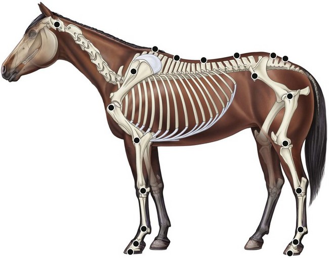
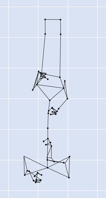
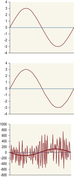
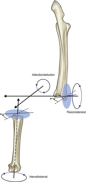
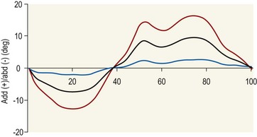
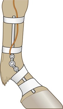
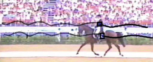
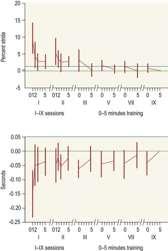
Chapter 2 In a qualitative evaluation of a horse’s gaits or movements, the human eye captures the image and the brain processes the information to form an opinion based on evaluating the observed motion in the context of previous experience. Even though some judges of horses and equestrian sports are very astute observers, subjectivity is inherent in this type of judgment. In assigning a lameness grade, clinicians draw on their powers of observation and previous experience to assign a lameness score in a semi-quantitative analysis. Experienced clinicians may be consistent in their scores (Back et al., 1993), but there is considerable variation between clinicians (Keegan et al., 1998). Variability is inherent to data obtained from repeated measurements on biological material. For example, when the horse is guided over the force plate, the chance for a correct hit by one fore hoof is about 50%, with the number of hits being approximately evenly distributed between the right and left limbs. After several runs, it is likely that a different number of correct hits will have been recorded from the right and left limbs. When calculating the mean and the standard error of the mean (SEM) for a force variable (e.g. peak vertical force) by averaging the data of these runs, the mean of the data obtained from the limb with the higher number of correct hits usually has a lower SEM. Are data from that limb more ‘correct’ than those from the other limb? Obviously not, but it is not easy to define a universal, statistically correct recipe to deal with this problem. In practice, most laboratories collect data until a certain minimum number of correct hits have been recorded from each limb. In sound horses, both the kinematic and force variables are quite stable, and analysis of three to five strides is sufficient to give a representative value for kinematic (Drevemo et al., 1980a) or GRF (Schamhardt, 1996) analysis. The mean value is then used in further stages of the analysis as being representative of that variable for a particular limb in one horse. Most of the stride variables show good repeatability over the short and long term (Drevemo et al., 1980b; van Weeren et al., 1993; Ishihara et al., 2005; Lynch et al., 2005), and the stride kinematics of a young horse have already assumed the characteristics that they will have at maturity by the time the foal is 4 months of age (Back et al., 1994). Some horses may, inherently, show more variability than others (Lynch et al., 2005) and variability may be affected by many of the conditions that are being studied, such as lameness, the presence of a rider and the fit of the saddle. Horses with more severe lameness tend to have larger coefficients of variation for kinetic variables, both within and between horses (Ishihara et al., 2005). On the other hand, variability in stride length increased significantly when lameness was reduced by intra-articular or perineural anesthesia (Peham et al., 2001). It was suggested that variations from the optimal motion pattern are associated with pain, so lame horses maintain a highly consistent kinematic pattern, whereas sound horses are not constrained by the association between kinematic variation and pain, so other influences on motion, such as external stimuli become more influential. In horses moving on a treadmill, variability in forward velocity and acceleration decreased when the horses were ridden but the same variables had higher variability when the rider used a poorly fitting saddle compared with a well fitting saddle (Peham et al., 2004). The treadmill is extremely useful for equine gait analysis due to the ability to control the speed of movement and the environment around the horse. It must be recognized, however, that stride kinematics on the treadmill differ in some respects from over ground locomotion (Fredricson et al., 1983; Barrey et al., 1993; Buchner et al., 1994b). Horses trotting at the same speed under both conditions use a higher stride frequency and a longer stride length on the treadmill (Barrey et al., 1993). The treadmill is also associated with longer stance durations, earlier placement of the forelimbs, greater retraction of both fore and hind limbs and reduced vertical excursions of the hooves and the withers (Buchner et al., 1994b). A period of habituation is required before horses move consistently on the treadmill, with habituation occurring more rapidly at faster gaits. Rapid adaptation is seen during the first few training sessions, and by the end of the third 5-min session, the kinematics of the trot have stabilized (Fig. 2.1), whereas walk kinematics are not fully adapted even at the tenth session (Buchner et al., 1994a). During the first session and, to a lesser extent at the start of subsequent sessions, the horse takes short, quick steps, with the withers and hindquarters lowered, and the feet splayed to the side to widen the base of support. Even experienced horses take at least one minute for their gait pattern to stabilize each time the treadmill belt starts moving (Buchner et al., 1994a). When measurements are made during treadmill locomotion, it is recommended that horses habituate for one minute after a change of gait or speed before making steady state measurements (Buchner et al., 1994a). Fig 2.1 Habituation to treadmill locomotion in 10 horses determined by changes in hind limb stance duration, expressed as a percentage of stride duration (above) and in seconds (below). The horizontal axis shows the number of training sessions, each of 5 min duration. The vertical axis shows the relative stance duration. Reductions in relative stance duration are regarded as a sign of habituation. The horizontal line indicates the ‘habituation limit’ based on data of the final recording session. Vertical bars indicate standard deviations within 10 horses. Reprinted from Buchner, H.H.F., Savelberg, H.H.C.M., Scharmhardt, H.C., et al., 1994. Kinematics of treadmill versus overground locomotion in horses, Veterinary Quarterly, Vol 16, supp2, S87–S90, with permission of Taylor & Francis Ltd, http://www.tandf.co.uk/journals. Horses moving on a treadmill use less energy than horses moving over ground at the same speed (Sloet & Barneveld, 1995), which may be partly due to a power transfer from the treadmill to the horse. Although the speed of the treadmill belt is assumed to be constant, in fact it is decreased by about 9% in early stance due to the frictional effect of the vertical force component and the decelerating effect of the longitudinal force component exerted by the horse’s hoof. Towards the end of the stance phase the frictional effect of the vertical force declines while the propulsive longitudinal force tends to accelerate the belt (Schamhardt et al., 1994). Kinematic analysis of horses moving on a treadmill has been used to study many aspects of equine locomotion, including movements of the limbs (Back et al., 1995a, 1995b), ontogeny of the trot (Back et al., 1994), response to training (van Weeren et al., 1993; Corley & Goodship, 1994), development of gait asymmetries (Drevemo et al., 1987) and kinematic adaptations used by the horse to manage lameness (Peloso et al., 1993; Buchner et al., 1995, 1996a, 1996b). The ability to incline the treadmill belt allows studies of stride kinematics when horses move on an incline or decline (Sloet et al., 1997; Hoyt et al., 2000; Dutto et al., 2004b; Hodson-Tole 2006). Mounted studies have also been performed on the treadmill, which provides a consistent speed and environment for assessing the influence of a rider (Barrey et al., 1993; Peham et al., 2004), the effects of different training techniques or riding styles (Gomez Alvarez et al., 2006; Weishaupt et al., 2006b) and the role of saddle fit (Peham et al. 2004; Meschan et al., 2007). Kinematic analysis quantifies the features of gait that are assessed qualitatively by visual evaluation in terms of temporal (timing), linear (distance) and angular measurements. Visualization of kinematic data is facilitated by constructing animated stick figures (Fig. 2.2) and by plotting the results graphically. Statistical analysis can be used to compare the entire curves (e.g. Deluzio & Astephen, 2007) or to compare discrete values that represent important events. Most motion analysis systems are based on tracking markers fixed to the skin or the bones. For two-dimensional analysis, circular markers, 1–3 cm in diameter are used, with bigger markers giving better accuracy when the resolution of the system is poor (Schamhardt et al., 1993a). Retroreflective material, which reflects light back along the same path as the incident light, can be purchased in sheets (Scotchlite, 3M Corp., St Paul, MN) and used to make markers of a suitable size or precut circles can be purchased at a higher price. Retroreflective paint (Scotchlite 7210 Silver, 3M Corp., St Paul, MN) is also available, but clumping of the reflective beads makes it difficult to use. When markers are fixed to the skin, they are usually attached over specific bony landmarks. Accurate palpation skills are a prerequisite. Inaccuracy in identification of anatomical landmarks is a major source of error in kinematic analysis (Weller et al., 2006). In order to minimize the inaccuracies, care should be taken that the horse is standing squarely with weight on all four limbs. Any change in position or loading of a limb alters the cutaneous relationship to the underlying bone. It is useful to mark the attachment sites on the skin or hoof wall to facilitate reattachment in the same place if a marker is lost during data collection or if markers are removed and replaced during sequential recording sessions. When markers fixed to the skin are used to represent motion of the bones, sliding of the skin over the bones introduces a significant source of error. In the proximal limb, the skin moves by as much as 12 cm relative to the bone in the sagittal plane (van Weeren et al., 1990b), which is sufficient to change the entire shape of the angle–time diagrams at the proximal joints (Back et al., 1995a). In the proximal limbs, uncorrected data cannot be used for absolute angular computations or for measuring muscle or tendon lengths based on limb kinematics. Correction for skin displacement may not be of primary importance in clinical applications, especially when comparing data in a repeated measures design, but it is essential in biomechanical applications when absolute values are important (van Weeren et al., 1992). Bone-fixed markers are usually attached via a Steinmann pin inserted percutaneously into the bone. A cluster of at least three tracking markers is rigidly attached to the pin immediately before data collection (Chateau et al., 2004, 2006; Clayton et al., 2004, 2007a, 2007b; Khumsap et al., 2004). Marker locations are chosen in accordance with the purposes of the analysis. Calculation of the angle between two limb segments in two dimensions requires a minimum of three markers: one over the center of joint rotation and one on each segment, preferably as far as possible from the marker representing the joint center. Figure 2.3 shows the approximate centers of joint rotation in the sagittal plane in the fore and hind limbs (Leach & Dyson, 1988). These locations are used with software that requires markers to be placed over the joint centers. An alternative technique uses two markers aligned along the long axis to represent the orientation of the segment with the difference between segmental angles being the joint angle. Ideally, marker locations should be easily identified by palpation and should be in sites where skin displacement relative to the underlying bones is minimal or correction algorithms are available for extracting the effects of skin displacement. Markers are placed on the dorsal midline of the back to evaluate trunk motion (Licka & Peham, 1998; Faber et al., 2002; Johnston et al., 2004). These trunk markers can also be used to check that the horse is moving straight and is aligned with the axes of the Global Coordinate System (GCS) during data collection (Fig. 2.4). Markers on the poll, withers and croup are useful for evaluating vertical excursions of these reference points and for detecting asymmetries associated with lameness (Buchner et al. 1996a; Keegan et al., 2004). Three-dimensional analysis requires a minimum of three non-colinear markers per segment. Ideally, the markers should be widely distributed over the segment and, as for two-dimensional analysis, placed in locations that show minimal skin displacement or for which correction algorithms for skin displacement are available. Each marker must be visible to at least two cameras throughout the movement and accuracy improves with an increase in the number of cameras tracking a marker. When markers are required in locations where they are difficult to track, it is possible to use a virtual targeting system (Nicodemus et al., 1999). This method relies on the fact that, for rigid body motion, the location of any point on a body does not change with respect to that body. Therefore, if the location of a point on a segment is known with respect to the position of the markers on that segment and the orientation of the segment is known in a GCS, then the location of that point on that segment can be calculated in the GCS. The virtual targeting method employs two sets of markers: tracking markers and virtual markers. Three (virtual or tracking) markers attached to each segment are used to define the segmental coordinate system: two are oriented along the long axis of the segment and the third is perpendicular to that axis. Three non-collinear tracking markers are placed on the segment in appropriate positions to track the motion of the segment in the GCS, i.e. at locations that are readily visible to the cameras during locomotion and at locations for which the skin displacement is known. A stationary file is recorded with both the virtual and tracking markers in place, after which the virtual markers are removed. Trials are recorded with only the tracking markers in place. In the sagittal plane, skin displacement relative to the underlying bones has been quantified and correction algorithms have been developed to calculate skin motion relative to specific bony landmarks from the scapula to the metacarpus and from the pelvis to the metatarsus of walking and trotting Dutch Warmblood horses (van Weeren et al., 1990a, 1990b, 1992). However, these algorithms are only valid for horses of similar conformation, moving at the same gaits and at similar speeds. For three-dimensional analysis, correction algorithms are available for sites on the crural and metatarsal segments (Lanovaz et al., 2004) and on the forearm segment (Sha et al., 2004) of trotting horses. The recording area or volume must be calibrated in order to scale the linear measurements. The accuracy of the calibration directly determines the accuracy of the final three-dimensional data (DeLuzio et al., 1993), which emphasizes the importance of investing the necessary effort into calibration of the volume space in which the measurements are made. During digitization small errors are introduced that constitute ‘noise’ in the signal. The effect of noise is not too great in the displacement data, but it becomes increasingly apparent in the time derivatives, i.e. the velocity and acceleration data (Fioretti & Jetto, 1989) as shown in Figure 2.5. Smoothing removes high-frequency noise introduced during the digitization process using one of two general approaches: a digital filter followed by finite difference technique or a curve-fitting technique (e.g. polynomial or spline curve fitting). Selection of an appropriate smoothing algorithm and smoothing parameter for a specific purpose requires some expertise and is discussed further in Chapter 3. As a guideline, a low-pass digital filter with a cut-off frequency of 10–15 Hz is adequate for most kinematic studies of equine gait. However, if the movement of a marker has an oscillatory component, as occurs when loose connective tissue is interposed between the skin and the underlying bones, these oscillations are essentially tied to the movements themselves and cannot be removed by smoothing (Schamhardt, 1996). Many kinematic variables are velocity-dependent. In designing research studies, consideration should be given to standardization of velocity. There are several ways in which this might be achieved. One method is to set a target velocity that all horses must adhere to within a predetermined, narrow range. This may be adequate when all the subjects are of similar size but is less satisfactory for horses that differ in size. On the treadmill, an energetically optimal speed can be determined at which the variation between motion cycles is minimized (Peham et al., 1998). This is a good method when performing repeated analyses of the same horse. However, if the protocol involves lameness, it is likely that the horse will have a slower preferred velocity when lame. An alternative approach to controlling the effects of velocity involves measuring velocity dependent changes in the variables, then developing a regression equation to predict the values of these variables at different velocities (Khumsap et al., 2001). Joint angles in the sagittal plane may be reported in terms of the absolute joint angle, which is usually measured on the anatomical flexor aspect of the joint. Alternatively, flexion (positive) and extension (negative) angles can be expressed relative to the position at which the proximal and distal segments are aligned. In some studies, joint angular measurements have been standardized to those obtained in the square standing horse (Back et al., 1994), so that the angles are reported as deviations from this square standing position (flexion positive, extension negative). Although the patterns are the same regardless of the method of measurement, the values differ considerably, which impairs comparisons between data from different studies. A drawback to reporting absolute values for kinematic variables is that conformational differences increase the variability between horses, which decreases statistical power and may make it difficult to detect real differences between experimental conditions. In a comparison of different methods of standardization for removing the effects of conformational variation, it was shown that subtraction of either the standing angle or the impact angle reduced variability without changing the data. Subtraction of the average joint angle during the trial or multiplicative scatter correction reduced variability even further but some of the variables changed significantly (Mullineaux et al., 2004) Horses vary greatly in size and to compensate for the effect of size, data can be scaled such that the kinetic and gravitational forces are proportional to the horse’s height and mass (Alexander, 1977). Temporal variables are adjusted for height at the withers using the equations for acceleration and velocity (Alexander, 1977). where height is subject height at the withers (m) and g is gravitational acceleration (9.8 m/s2). Similarly, subject velocities are standardized by dividing measured velocity by adjusted velocity and expressed as velocity in dimensionless units (VDU). An objective method of predetermining an equivalent velocity for horses of different sizes is to adjust the velocity on an individual basis by taking into account height at the withers and the effects of gravitational acceleration as described above (Alexander, 1977). After setting the VDU, the target velocity for each horse is calculated. GRFs are standardized to the subject’s body mass and expressed as force per kg body mass (N/kg). Impulses are affected by both mass and height at the withers. The measured impulse (force*stance duration) is divided by the force due to body mass (weight*g) multiplied by the adjusted time, and expressed as the impulse in dimensionless units (IDU). The equation to obtain IDU is: An approach that has been used in some equine studies is to project the three-dimensional coordinate data onto three orthogonal planes that are tied to the GCS (Fredricson & Drevemo, 1972). Provided the horse moves in a direction parallel to a global coordinate axis, the analytic planes become the sagittal (side view), frontal (front or rear view) and dorsal (dorsal or ventral view) planes. In effect, this method degrades the three-dimensional analysis into a series of quasi-two-dimensional analyses. Joint motion that is not parallel to one of the projection planes cannot be accurately measured and, since the segments are defined as simple lines between landmarks, rotations along the long axis of a segment are impossible to measure. A true three-dimensional analysis requires multiple cameras that are synchronized precisely and with each marker visible to at least two cameras at all times. Each length measurement has three components in space and a segment requires three angle measurements to define its orientation. A three-dimensional joint coordinate system (JCS) is established for the joint based on embedding an anatomically meaningful coordinate system within each limb segment comprising the joint. Flexion/extension, adduction/abduction, and internal/external rotation are usually expressed as motions of the distal segment relative to the fixed proximal segment (Fig. 2.6). The angles can be described independently of each other, which allows for examination of complex coupled motion in a joint. Angles measured with the JCS are independent of the joint centers of rotation. One method of expressing three-dimensional joint motions is based on a strictly ordered sequence of three rotations, known as Euler angles. In aeronautical terminology these are referred to as pitch, yaw and roll. The drawback to the use of Euler angles is the need to specify the order of rotations. In an effort to express joint motion in a context that is more meaningful to clinicians, Grood and Suntay (1983) proposed the use of a JCS for the human knee joint in which the rotations are consistent with the clinical definitions of flexion/extension, abduction/adduction and internal/external rotation. The first axis of rotation (flexion/extension) was attached to the segment proximal to the joint, the third (internal/external rotation) axis was attached to the distal segment and the second (adduction/abduction) axis was a floating axis that was mutually perpendicular to the other two axes and was not aligned with the planes of either segment (Fig. 2.6). For each axis, there is a rotation around the axis and a translation along the axis. All three rotations take place at the same time, as in a mechanical linkage, thus eliminating the need to specify the order of rotations. The method of Grood and Suntay (1983) brought a wider acceptance of the value of the JCS in a clinical setting, though it is now understood that their method is actually identical to the Euler angle method. When using the JCS method, kinematic analysis is typically performed in three steps. The first step is to define a coordinate system on each bone. Second, the rotation matrix and translation vector relating the GCS with the JCS is obtained from three-dimensional marker coordinates during motion using a singular value decomposition method (Soderkvist & Wedin, 1993). This algorithm produces a rotation matrix and a translation vector that describe the rotation and translation of the segmental coordinate system from its neutral position in the stationary file to the orientation in each frame of tracked data. In the final step, matrix equations are used to extract the three rotation angles and three translations (Grood & Suntay, 1983). Relative angular motions (helical angle changes) between the segments may be calculated using a spatial attitude method (Spoor & Veldpaus, 1980; Woltring, 1994) or Euler angles may be calculated (Ramakrishnan & Kadaba, 1991). Software is available to perform these steps or computer code can be accessed in the public domain. Markers on the model are defined and, from the marker trajectories, joint rotations and translations are solved iteratively by global optimization. When using a segment-based or bone-based local coordinate system, decisions regarding the establishment and orientation of the axes have important effects on the results of the analysis and must, therefore, be stated clearly (Capozzo et al., 2005). Both joint kinematics (Beardsley et al., 2007) and net joint moments (Schache & Baker, 2007) vary significantly according to the coordinate system used and, even though the alternative frames of reference are mathematically valid, differences in output affect interpretation of the results. Clinical conclusions can be upheld or refuted, based on the same data set, subject to coordinate system definitions (Beardsley et al., 2007). Choice of the coordinate system is, therefore, critical to the outcome of a study. In equine studies, limb segment axes have been based on anatomical landmarks identified by palpation and/or fluoroscopy (Khumsap et al., 2004; Clayton et al., 2004, 2007a, 2007b) or using a template attached to the bones (Chateau et al., 2004, 2006). A right-handed coordinate system is used to establish the three axes around which flexion/extension, abduction/adduction and internal/external rotation occur. Errors are reduced if the axis aligned with the longest dimension of the bone is established first. Kinematic crosstalk is a common problem in using the JCS method. Flexion/extension angles are robust due to their large signal to noise ratio and misalignments between the horse or the plane of motion and the GCS tend to have little effect on flexion/extension measurements where this is the predominant type of motion (Ramakrishnan & Kadaba, 1991). However, these misalignments will cause some of the flexion movement to be misinterpreted as abduction. Figure 2.7 shows the effect of a small (±10°) change in alignment of the flexion/extension axis on the amount of motion ascribed to abduction/adduction at the fetlock joint (Clayton et al., 2007a). Another problem with the JCS methodology is gimbal lock, which causes the rotation angles to become increasingly sensitive to measuring errors when the second rotation approaches ±90° (Woltring, 1994). An electrogoniometer or elgon is a device for measuring joint angle changes. It consists of a potentiometer attached to two rigid, rotating arms that are fixed to the limb with tape or straps, so that the center of the elgon lies over the center of rotation of the joint (Fig. 2.8). A change in joint angle alters the electrical resistance of the potentiometer, which is calibrated with a protractor. Permanent records, or goniograms, can be recorded on an oscilloscope and the data stored for later analysis. In horses, electrogoniometry has been used to record joint movements at different gaits in normal and lame horses (Adrian et al., 1977), to diagnose obscure lameness, and to evaluate changes in joint motion after medical or surgical treatment (Taylor et al., 1966; Ratzlaff et al., 1979). The availability of image-based motion analysis systems has superseded the use of electrogoniometry. A standard camcorder records 30 frames/s in the NTSC format and 25 frames/s in the PAL format. Each frame consists of two interlaced video fields recorded 1/60 s (NTSC) or 1/50 s (PAL) apart. Software displays successive fields sequentially giving an effective sampling rate of 60 fields/s (NTSC) or 50 fields/s (PAL). High-speed video cameras are useful for studies of short-duration events or rapid movements but the lighting conditions become critical at faster recording speeds. Comparisons of joint displacement data from horses cantering on a treadmill showed minimal loss of information in terms of angular data when the sampling rate was reduced from 200 Hz to 50 Hz (Lanovaz, unpublished). Linford (1994) compared the temporal stride variables in horses trotting on a treadmill by analyzing the same ten strides with cameras sampling at 60 Hz and 1000 Hz, respectively. Mean values for stride duration, stance duration, swing duration, and breakover did not differ by more than 3.3 ms. Thus, 60 Hz is an adequate sampling rate for kinematic analysis of many aspects of equine locomotion, but a large number of strides must be analyzed to produce a representative mean value for temporal events of short duration. At gaits faster than a walk, a higher sampling rate is preferable, especially if the displacement data will be processed further. A number of software packages with varying levels of sophistication are marketed for video-based kinematic analysis. These packages may offer marker-less tracking, simultaneous multiple two-dimensional video capture and stroboscopic imaging. Marker-less tracking digitizes unique user specified patterns on a frame-by-frame basis without markers or manual intervention. If the image contains a distinguishable pattern that is visible across several frames, the system can recognize a point within the pattern and track it automatically for the entire sequence (Fig. 2.9). By simultaneously collecting multiple two-dimensional camera views, it is possible to perform a multi-planar analysis. Images that represent distinct events, such as ground contact, midstance and lift-off, can be viewed to create stroboscopic files. The majority of equine gait labs use digital optical motion capture systems that offer automatic marker identification with real-time processing of the three-dimensional coordinates to display graphs and stick figures of the motion and other types of calculated data during or immediately after the movement occurs. Other sources of analog or digital data from force platforms, EMG systems, dynamometers, foot switches, event recorders, etc., can be synchronized with the system. Kinematic data may be recorded using active markers (markers that emit a signal) or passive markers (markers that detect or reflect a signal). Most of the equine gait laboratories currently use optoelectronic systems based on passive markers, such as the Motion Analysis System (Motion Analysis Corp., Santa Rosa, CA), Vicon MX (Vicon, Oxford, UK) or ProReflex MCU (Qualysis Inc., Glastonbury, CT). Figure 2.10 shows data collection in progress using a Motion Analysis System in the Mary Anne McPhail Equine Performance Center at Michigan State University. Electromagnetic systems, such as Flock of Birds (Ascension Technologies, Burlington, VT) are used as three-dimensional tracking devices for applications that include real-time visualization, and target acquisition. The magnetic tracking has accuracy comparable with an optical motion system (Hassan et al., 2007). Drawbacks to the use of an electromagnetic system include the problem of metal interference, the relative heaviness of the receivers, the presence of wires and the small data capture volume. An ultrasonographic system for real-time, three-dimensional gait analysis (Zebris CMS-HS, Medizintechnik Gmbh, Isny, Germany) is based on temporal delay of ultrasound signals. The system uses marker triads consisting of three small ultrasound microphones (Fig. 2.11) that operate sequentially and are mounted at a predetermined distance from each other (Fig. 2.11). The position of the markers is determined relative to a fixed system of three ultrasound transmitters and the x, y, z coordinates of the markers are determined by triangulation, based on the delay in the ultrasound pulses. In standard laboratory conditions, the precision of the Zebris system was measured as ±0.14 mm for linear measurements and ±0.16° for angular measurements, but the precision decreased if the distance between the transmitters and the microphones exceeded 1.5 m. This restricts the size of the data collection volume and does not permit recording of data for a complete stride during over ground locomotion (Chateau et al., 2003). Although the maximum sampling frequency is 100 Hz, the relationship between sampling rate, measuring distance and time between ultrasonic pulses is such that a sampling frequency of 50–60 Hz is practical for equine studies (Chateau et al., 2003). Ultrasound reflections can induce systematic errors (about 0.2°) and impair the repeatability of the measurements. Wind decreases the precision of the measurements in proportion with its speed and temperature also has an effect, so it is necessary to configure temperature in the software. This system has been used in precision analysis of the stance phase of horses walking and trotting over ground and in analysis of the stance and swing phases of horses walking and trotting on a treadmill (Chateau et al., 2004, 2006). Kinetic analysis measures locomotor forces, both external and internal to the body. Forces developed by muscles are transformed into rotations of the limb segments that ultimately produce movement. The forces between the hoof and the ground during locomotion can be recorded using a force plate (e.g. Pratt & O’Connor, 1976; Seeherman et al., 1987; Merkens et al., 1988, 1993a, 1993b; Dutto et al., 2004b) or a force shoe (Björck 1958; Frederick & Henderson 1970; Hjertén & Drevemo, 1987; Barrey, 1990; Ratzlaff et al., 1990, 1994; Keg et al., 1992; Roepstorff & Drevemo, 1993; Kai et al. 2000; Rollot et al., 2004; Roland et al., 2005). Transmission of forces and accelerations through the body are recorded by strain transducers, ultrasonic transducers, accelerometers, gyroscopes and magnetometers attached directly to the segment. During the stance phase of the stride, the hoof exerts a force against the ground and, according to Newton’s third law of motion, the ground exerts a reaction force against the hoof that is equal in magnitude and acts in the opposite direction. This ground reaction force (GRF) is fully described by its magnitude, direction and point of application. To aid in understanding the effects of the GRF, the three-dimensional force vector may be resolved into components acting in the vertical, longitudinal (craniocaudal), and transverse (mediolateral) directions. When the frame of reference changes, for example if the horse moves on an incline or decline, the components may be aligned with the ground rather than the global reference frame (Dutto et al., 2004b). Measurement devices may provide complete three-dimensional data or a more limited range of GRF components, so the method of measurement should be chosen in accordance with the goals of the study. Standard GRF patterns have been developed for Dutch Warmbloods at a walk (Merkens et al., 1988), trot (Merkens et al., 1993a) and canter (Merkens et al., 1993b). Since there are significant differences between breeds (Back et al., 2007), the Dutch Warmblood data must be adapted to other breeds by incorporating appropriate parameters and weighting factors into the formulae used to develop the standard patterns. For example, when forces are normalized to body weight, Quarter Horses have lower vertical GRFs than Dutch Warmbloods trotting at a similar velocity (Back et al., 2007). Figure 2.12 shows the three force components (vertical, longitudinal, transverse) during the stance phase of a forelimb at a walk and trot. The vertical force, which represents the anti-gravity support function of the limb, is always positive. The longitudinal force, which provides acceleration and deceleration, has negative and positive phases. In the early part of the stance phase, the longitudinal force brakes (decelerates) the horse’s forward movement as a result of friction that prevents the hoof slipping forward. Later in the stance phase, it changes to a propulsive (accelerating) force. The direction of the horse’s motion across the force plate determines whether acceleration or deceleration is recorded as positive. Software correction is applied to standardize the sign convention. The transverse force, which increases during sideways or turning movements, is small in magnitude when moving in a straight line and is directed medially. The left to right values recorded by the force plate can be converted during post-processing to represent medial and lateral values for each limb. During turning the transverse force acts toward the center of the turn or toward the direction of lateral motion.
Measurement techniques for gait analysis
Introduction
Interpreting the effects of biological variability
Treadmill evaluation
Kinematic analysis
Markers
Calibration
Smoothing
Normalization


Multi-planar analysis
Three-dimensional analysis
Methods of kinematic analysis
Electrogoniometry
Photographic systems
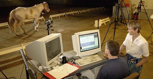
Optoelectronic systems
Electromagnetic systems
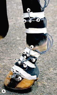
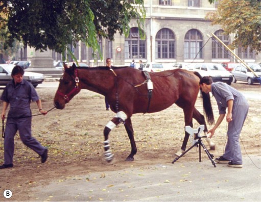
Ultrasonographic system
Kinetic analysis
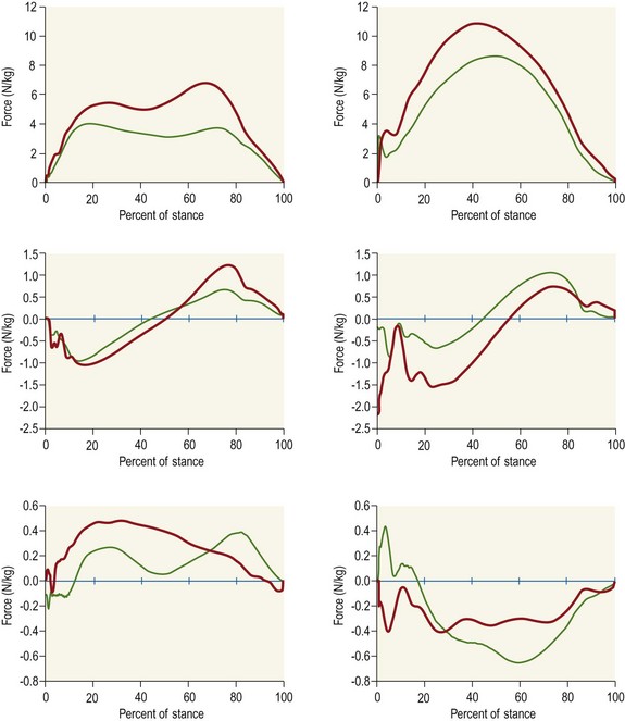
Ground reaction force
Measurement techniques for gait analysis