The Role of Computed Tomography and Magnetic Resonance Imaging in Veterinary Practice

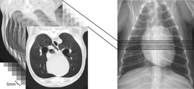
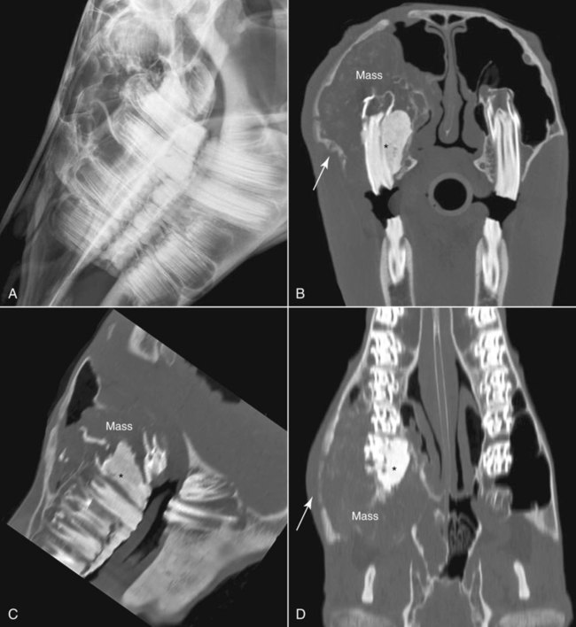
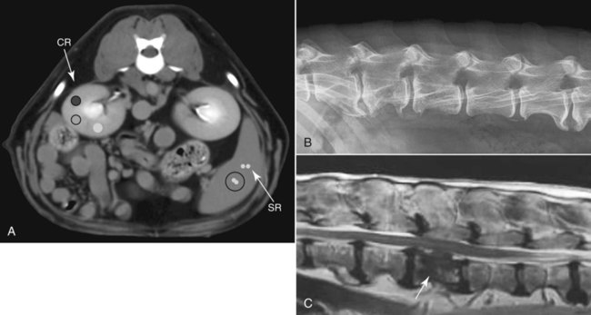
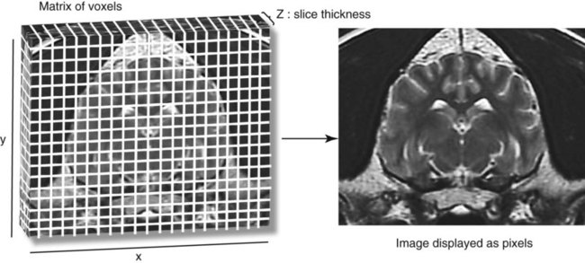
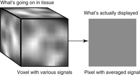
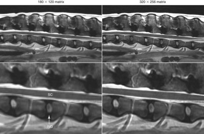
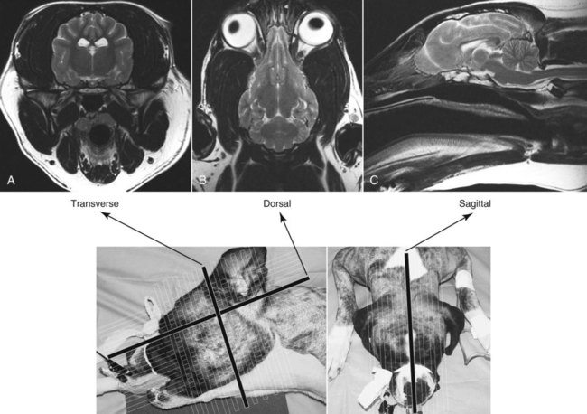
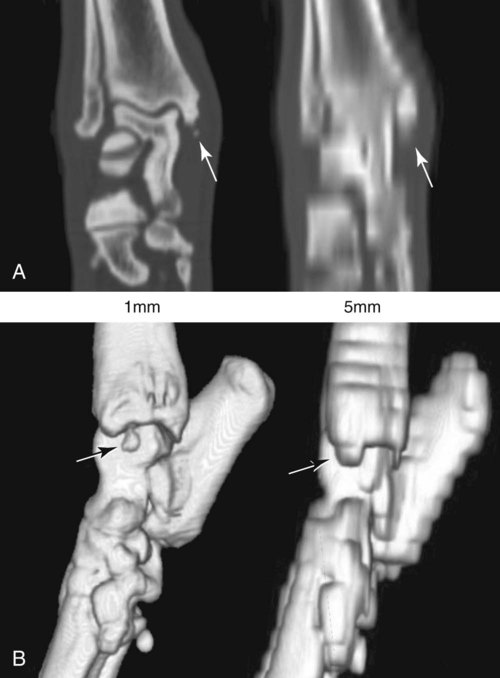
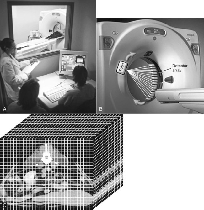
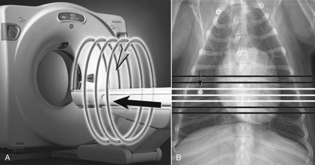
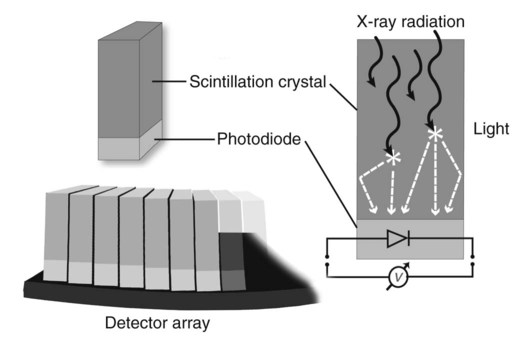
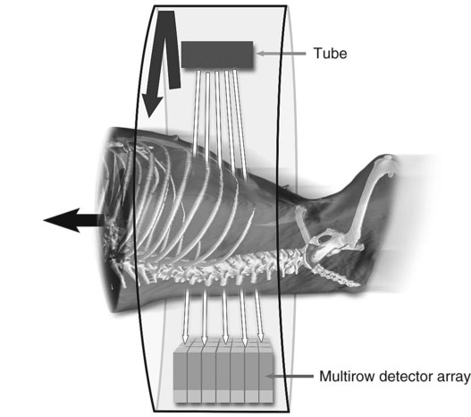
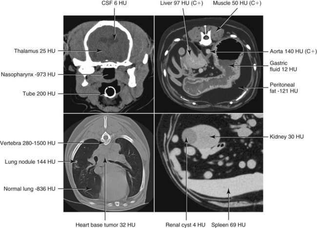
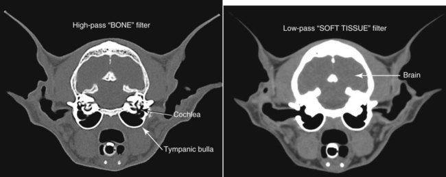
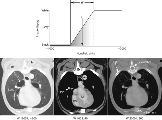
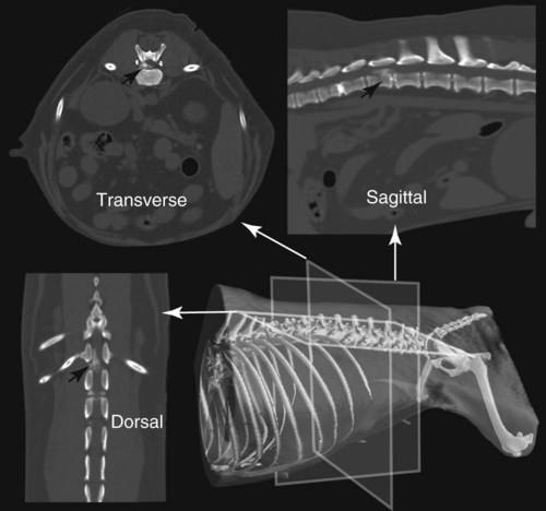
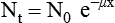
CT and MR imaging offer superior diagnostic possibilities over conventional radiography because of two primary advantages, which are their tomographic nature and increased contrast resolution. Indeed, as opposed to radiographs that represent two-dimensional, or flat, projections of three-dimensional structures, tissues are examined with CT and MR in thin sections, or slices, thereby eliminating superimposition. Organs and other structures can then be identified more easily and differentiated (Figs. 4-1 and 4-2). Moreover, CT and MR volume datasets can be reformatted in any imaging plane, or as three-dimensional (3-D) projections, allowing better representations of structural anatomic relationships.

Contrast resolution is the capacity of a system to accurately represent differences in tissue, physical, and/or biochemical characteristics, which are intrinsically linked to x-ray attenuation (CT) or signal intensity (MR). The better the contrast resolution, the more likely subtle variations in tissue components will be displayed as pixels of different shades of gray, whether these components are normal or pathologic (Fig. 4-3, A). For example, differences in x-ray attenuation as little as 0.5% can be identified with CT, as opposed to approximately 5% on a radiograph.¹ This difference is mainly explained by the virtual elimination of scatter that reduces contrast on radiographs.² As with ultrasonography, pure liquids can be differentiated from soft tissues with CT, which cannot be done with radiographs. MR imaging is recognized even more for its great contrast resolution (Fig. 4-3, B), which can be enhanced by the combined use of different imaging sequences.

Conversely, spatial resolution, which corresponds to the minimum resolvable separation between high-contrast objects (see Fig. 4-3, A), is relatively limited with CT and MR imaging, as opposed to radiography. The spatial resolution of CT and MR imaging, which is typically linked to the slice thickness, is approximately 0.4 and 1.0 mm,³ respectively, although technical advances and increased magnetic field strength have contributed to reducing this value for MR imaging. In comparison, screen-film and digital radiography are associated with a spatial resolution of approximately 0.08 to 0.17 mm,³ which allows smaller details to be depicted. However, the elimination of superimposition and superior contrast resolutions inherent to CT and MR imaging more than compensate for this limitation.

Image Formation: General Concepts

CT and MR imaging share several characteristics regarding image formation. Each generated image represents a thin section, or slice, of the body, composed of a matrix filled with small cubical sections, known as voxels, or volume elements, which is displayed on a flat monitor as a matrix of pixels, or picture elements (Fig. 4-4). For both CT and MR imaging, each voxel of the matrix is associated with an electronic current that is spatially localized in the body and processed by a specialized computer system. Variations in electronic current intensity are expressed as variable pixel brightness on a monitor. Thus, a voxel associated with greater tissue signal intensity on MR or x-ray attenuation on CT will be displayed as a brighter, or whiter, pixel, whereas lack of signal or x-ray attenuation, such as with air, will appear dark. Although several different values can coexist in each voxel, especially if the voxel is large and if composed of heterogeneous tissue components, only the mean value is expressed and converted to pixel brightness (Fig. 4-5). The image grayscale is then determined by the range of brightness values filling each matrix.

This concept of voxel-to-pixel translation is intimately related to spatial and contrast resolution, which were discussed earlier. Indeed, a large voxel can contain tissue composed of smaller elements of different morphologic and biochemical characteristics. Hence, both normal and abnormal tissue elements may be combined in a voxel, limiting the resolving capabilities of the modality. Generally, the limiting factor with CT and MR imaging is the slice thickness, which is typically the largest dimension of each voxel. Much of the technical advances aim to reach isotropic resolution, that is, to image sections of tissue with perfectly cubical voxels— the x, y, and z dimensions are the same.² Figure 4-6 illustrates the impact of voxel dimension on image detail.

Among the differences between CT and MR imaging, an important aspect is that image sections can be acquired in any plane with MR imaging (Fig. 4-7). That is, images can be obtained in transverse, sagittal, dorsal, or any oblique plane. Conversely, with CT, images can be acquired only parallel to the system gantry. Thus, images are typically transverse to body parts lying on the CT table. Fortunately, sections are scanned contiguously, forming a volume dataset of millions of tiny cubes, each associated with an attenuation value. It is therefore possible to rearrange, or reformat, images so that voxels along a plane different than the transverse plane are now displayed as a new matrix of pixels (Fig. 4-8, Video 1). This process is known as multiplanar reformatting. These new images can assist in structure recognition, especially when tubular or tortuous, and allow more complete assessment (measurements, etc.) of normal and abnormal tissues. Moreover, imaging software can be used to generate 3-D representations through volume or surface rendering methods, helping clinicians, especially those less familiar with tomographic imaging, better understand morphologic changes and plan surgery. Although these manipulations can be performed with any CT dataset, the quality of reformatted or 3-D images is influenced by the initial image spatial resolution, and mainly its slice thickness. For example, transverse images obtained from 5- to 7-mm-thick sections, once reformatted along the sagittal or dorsal planes, will be associated with steplike contour artifacts (Fig. 4-9). Conversely, image reformatting using 0.62 mm-thick sections (i.e., nearly isotropic resolution) will generate images of structures with smoother contours. This represents an important benefit of multirow detector technologies. Although this level of resolution may not always be necessary, it can exert an impact on diagnostic accuracy, especially when very small structures (e.g., bone fragments, lung nodules) are imaged.

Computed Tomography

In 1979, G. N. Hounsfield and A. M. Cormack were awarded the Nobel Prize in medicine for the invention of CT,¹ which was considered by many to be the greatest advance in medicine since the invention of radiography. Individual images that took several minutes to acquire and reconstruct with sophisticated computers back then can now be generated in fractions of a second, significantly expanding the range of diagnostic applications while improving patient comfort and reducing motion artifact.

CT technology was based on Radon’s mathematic principles developed in 1917, which proved that an image of an object could be produced by the use of an infinite number of projections through that object.¹ With conventional radiographs, orthogonal projections are used to mentally reconstruct anatomic structures in 3-D based on the visualization of their shape on perpendicular projections. This process is reliable for simple shapes, but to represent structures with irregular contours accurately, many more projections are necessary. Now, if thousands of projections could be performed at precise angles, and if x-ray transmission through tissues could be quantified for each of these projections, a sophisticated computer would be able to geometrically reconstruct these data and assign specific x-ray transmission values to individual regions of the body. By using a thinly collimated x-ray beam rotating around a patient, slices of tissues can then be computerized, each with its own matrix of voxels associated with definite attenuation values. This is the fundamental concept of CT.

Computed Tomography System Geometry

A CT system is mainly composed of a scanning unit (i.e., the gantry) with a rotating x-ray emitting tube and a detector system, a patient table, and a console equipped with a sophisticated computer that allows adjusting acquisition parameters and image reconstruction (Fig. 4-10). The rotating x-ray tube is powerful enough to operate for long periods of time without overheating, thus permitting acquisition of large volumes of data. Initially, information could be obtained only one slice at a time because of the wire joining the rotating tube to the stationary electric circuitry in the gantry. Thus, the tube was rotated back to its original position after each scan, introducing an additional delay between each image acquisition. Slip-ring electromechanical devices, consisting of circular electrical conductive rings and brushes allowing the transmission of power from the stationary circuitry to the rotating tube, were then developed to allow uninterrupted tube rotation. Along with the concurrent development of high-capacity x-ray tubes, the introduction of slip-rings opened the door to helical (or spiral) scanning, a revolutionary advancement in CT imaging (Fig. 4-11, A). With the traditional sequential, or slice-by-slice mode, a cross-sectional image is produced by scanning a flat, transverse slice of the body of a patient lying on a stationary table. Because of body motion that may be difficult to control (e.g., respiration or peristalsis), images may not be consistent with the patient anatomy, leading to tissue misregistration. For example, a small lung nodule may not be detected if it moves because of respiration during sequential scanning (Fig. 4-11, B). With helical scanning, however, an entire body region, or the whole body, can be imaged without interruption and at greater speed, eliminating such acquisition gaps. Helical scanning is possible because of concurrent table advancement into the gantry as the tube rotates around the patient, which then traces a helical path around the body and produces a data volume rather than a single slice. Using interpolation methods, flat slices of cubical voxels can be reconstructed from any part of the dataset. Additionally, helical scans are performed much faster, reducing motion artifact and allowing angiographic procedures that require precise contrast-medium bolus tracking. Moreover, because of the geometry of helical scans, multiplanar and 3-D reformatting are less prone to steplike artifacts, resulting in smoother images. For these reasons, helical scanning is the standard in veterinary medicine, although sequential scans are also performed when motion is less an issue (e.g., scanning the head) and to prevent tube heat overload.

The detector system also plays an important role in image quality. It converts the incident x-rays that traverse tissue into electronic signals. Ceramic, solid-state detectors have better x-ray absorption and are used in current systems.1,4 Each detector is composed of a scintillation crystal that reacts with the incident x-ray, and through an amplification process, generates light that is converted into digital pulses (Fig. 4-12). Detectors are aligned over a semicircular (generally 60 degrees) or annular (360 degrees) array, depending on the system geometry. Annular arrays are stationary, whereas semicircular arrays move synchronously with the opposing x-ray tube (see Fig. 4-10, B). Although most CT scanners used currently in veterinary practices are of single-row configuration, multi-row detectors are increasingly available (Fig. 4-13). The use of very thin slices with single-row scanners is limited by the fact that only one slice is imaged at a time. For example, 5 mm-thick slices of a 30 cm-long thorax, imaged helically at a pitch of 1 and with a tube rotation of 1 second, would require 60 seconds to image, which is far better than conventional section-by-section scanning, but still difficult to achieve without respiratory motion. Multi-row detectors use radiation delivered from x-ray tube more efficiently than single-row detectors. By simultaneously scanning several slices, scan times can be reduced significantly, or the smallest details can be scanned within practical scan times.² This improves the quality of angiographic procedures such as those used for portosystemic shunt detection.

Image Formation

CT images are composed of pixels that, as discussed earlier, represent the mean attenuation values attributed to the corresponding boxlike tissue elements (i.e., voxels). The mechanism by which the system reconstructs the data measured by each detector as the tube rotates around the patient is sophisticated, yet relatively simple. It starts with the concept of x-ray attenuation, which mainly depends on the electron density of the medium. X-ray attenuation is quantified by measuring the fraction of radiation removed in passing through a given thickness of a specific material. The absorption probability is described by the linear attenuation coefficient (µ). Attenuation results in removal of x-ray photons according to equation (1)⁵:

Nt=N0e–μx (1)

(1)

where N₀ is the number of initial photons (detected at the tube exit), N_t is the number of transmitted photons measured by the detector, e is the base of the natural logarithm (2.718), x is the thickness of the absorber, and µ is the total linear coefficient of all tissues present along the x-ray path (called ray). After rearranging this formula, µ can be derived because N₀ and N_t are measured in the system, and e and x are known. This mathematic process is complicated by the fact that, for a single CT image, approximately 800 transmission measurements are obtained at 1000 different projection angles (fan-beam geometry), for a total of approximately 800,000 transmission measurements. Once µ is measured for a signal ray, the µ of each individual voxel composing the image matrix can be determined, generally using another mathematic process called filtered backprojection. Practically, for a single image with a 512 × 512 pixel matrix, this represents 262,144 different µ values. For display purposes, these values are transformed into Hounsfield units (HU) or CT numbers, normalized to voxel values containing water (µ_w). HU for other tissues are then calculated from Equation (2):¹

HU of a tissue=[(μtissue−μw)/μw]×1000 (2)

(2)

Based on this formula, the HU of pure water is zero, and any structure causing more x-ray attenuation than water will have a HU value above zero, whereas hypoattenuating media will have a HU value less than zero (negative). Figure 4-14 illustrates the range of HU among normal and abnormal tissues. The fact that liquids and soft tissues can be discriminated based on their HU values confirms the greater contrast resolution of CT over radiography.

Other important parameters that are set before image reconstruction include slice reconstruction interval, which adjusts the proportion of overlap between adjacent slices of tissues used for image reconstruction, and reconstruction filter, which determines the level of edge reinforcement applied while processing raw data. These parameters must be set carefully according to the region of interest. For example, a low-pass filter, commonly known as “standard or soft tissue filter” is recommended when soft tissue contrast must be emphasized, such as in brain imaging, with the downside of creating blurry images (Fig. 4-15). “Bone filters,” conversely, maximize spatial resolution, but introduce more noise, thus reducing contrast resolution. Such images are sharper but grainier

Image Display

HU values that can be measured with typical scanners range from approximately −1000 to +3095 HU, for a total of 4096 shades of gray (12 bits of grayscale*). This range of values cannot be resolved by the human eye, which cannot differentiate more than 90 shades of gray.¹ To visualize and appreciate all tissues composed of variable HU, the window width (W) and level (L) of the image grayscale must be adjusted, according to the median and range of HU composing the area of interest. The DICOM viewing software allows adjustment of the extent (maximum-to-minimum) of gray shades (W) displayed (i.e., the image contrast) and the HU at the center of the window (L) (Fig. 4-16, Video 2). W/L must be adapted to the tissues evaluated and usually requires several adjustments during an examination for all tissues to be evaluated completely.