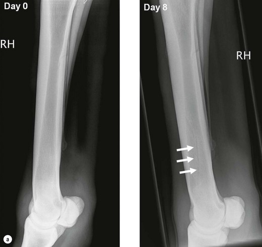
Chapter 25 • X-rays are electromagnetic waves from the high-energy end of the electromagnetic spectrum (visible light or radiowaves are part of the same spectrum, but of lower energy and different wave length). • X-rays are produced when fast moving electrons collide with matter. This happens in an X-ray tube that houses a cathode and an anode. By heating up the cathode, a cloud of electrons (negatively charged particles) is produced, which are accelerated till they hit the positive anode at high speed. • The higher the temperature of the cathode the more electrons are produced; this is related to the mAs (milliAmpere seconds) settings of the X-ray machine. • The higher the speed of the electrons the higher the penetrating power of the resulting X-rays. This is controlled by the kV settings of the X-ray machine. • X-rays radiate from the source in straight lines in all directions. For medical purposes only a small cone of the X-rays, the primary beam, is used. • The size of the primary beam is set by adjusting the window through which X-rays can leave their housing. This is called collimation and is an essential radiation protection mechanism, but also optimizes image quality by reducing scatter. • The intensity of the X-ray beam is inversely proportional to the square of the distance from the source. This is obviously important for radiation safety consideration and has to be taken into account when adjusting exposure settings: • When X-rays hit matter, they can either penetrate the material or get absorbed by it. The main underlying principles on an atomic level are called the Compton and the Photoelectric effect. The Compton effect is less desirable because it is responsible for scatter radiation that degrades image quality. • The degree of absorption is determined by the thickness and the radiodensity of the absorber. • The radiodensity depends on the physical density and the atomic number of the material, e.g. lead has a very high atomic number which allows complete absorption of X-rays with only a few millimetres of material. This is the reason why lead is used for shielding purposes, e.g. in protective clothing. The same effect can be achieved with material of lower atomic number, by increasing its thickness, e.g. a 20 cm brick wall. • The body is composed of materials of different radiodensities and thickness, hence X-rays are absorbed differentially. For example bone has a higher radiodensity and hence absorbs more X-rays than does soft tissue. This provides the basis for the image contrast that allows differentiation between structures on radiographs. • While the way X-rays are generated has not changed much, the way they are detected has undergone considerable changes in the last few years. • Conventionally, X-rays are detected using photographic film in combination with intensifying screens. After exposure the film needs developing in a similar process to film-based photography, to produce the final radiograph. More and more practices, however, now use computerized radiography (CR) or digital radiography (DR). • CR systems still require the use of cassettes and a processor. A phosphor-coated plate in the cassette absorbs X-rays and stores them as energy. The stored energy is released as visible light after stimulation of the atoms on the phosphor plate with a laser beam in the processor. The light is registered and converted into a digital signal. After erasing the imaging plate, it can then be re-used. • In DR systems the image is displayed directly on a screen without the necessity of processing a plate. • Image resolution quantifies how close structures can be to each other and still be visibly resolved and provides a measure of detail. In radiography it is usually expressed as line pairs/mm. • Image contrast is the difference in radiodensity that makes an object distinguishable from another structure. • Exposure latitude is the extent to which a radiograph can be over- or underexposed and still achieve an acceptable result. • Decreasing the kV settings increases the image contrast, but decreases the latitude. For each 10 kV change the mAs setting has to be doubled or halved to maintain the same opacity. A kV setting under 70 is desirable for good bone radiographs. • Image sharpness describes how well the edges of a structure can be distinguished from other structures or the background. It is influenced by the. • Bone is a dynamic tissue and undergoes constant changes in response to the stress it is put under (Wolff’s law). This results in changes in bone density and bone shape, which is a physiological process but changes with pathology. • A 30–50% change in mineralization is required before it can be visualized on radiographs. • Compared to other species (e.g. humans and dogs) the horse has a very slow bone metabolism, hence radiographic changes are slow to develop. • Once radiographic abnormalities have developed they can persist for a long time without being significant. • Periosteal new bone: often caused by trauma, but can also be caused by infection (Figures 25.1, 25.2, 25.3). • Endosteal new bone: most commonly associated with trauma, e.g. fractures, but can also be caused by infection or inflammation. • Cortical thickening: in response to stress. • Callus formation: fracture repair (Figure 25.3). • Enthesiophytes: focal, distinct new bone formation at attachment site of ligaments, tendons and joint capsule, usually associated with chronic strain at this site (Figures 25.4, 25.5, 25.6). • Osteophytes: periarticular new bone usually associated with osteoarthritis (Figures 25.4, 25.6, 25.7). • Sclerosis is a term used for localized new bone formation, usually in response to stress (e.g. subchondral bone sclerosis in osteoarthritis) or when the body is walling off areas, e.g. a sequestrum or bone cyst) (Figures 25.1, 25.7, 25.8, 25.9). • Radiographs are not very sensitive when it comes to the assessment of different soft-tissue densities: e.g. fluids such as blood or urine have the same radiographic appearance as most soft tissues (tendons, cartilage etc.). • The exception is fat, which appears more radiolucent than other soft tissues, which can, for example, be appreciated in the case of the triangular radiolucency consistent with the patellar fat pad in the stifle (Figures 25.11, 25.12). • Confirm a clinically suspected diagnosis. • Assess the severity of a disease. • Exclude other pathological conditions. Pitfalls in radiographic interpretation • Over-interpretation: detecting pathology where none is present: • Under-interpretation: missing lesions. • Radiographs should be displayed on a viewing box in the case of films and a hot light should be available to highlight areas. Holding radiographs against the sun is not acceptable! • In the case of digital images, a high-resolution screen should be used and one should ensure that the image format does not involve compression, and hence loss of quality. A standard approach should incorporate the assessment of the following parameters: • Assessment of diagnostic quality. The first step in interpreting radiographs is to decide whether or not the radiographs are of diagnostic quality. The following parameters should be evaluated: • Identification of subject: species, age (skeletally mature/immature). Table 25.1 shows the radiographic closure times for growth plates in the horse. • Description of a lesion by its Röntgen signs. • Conclusion. Lesions should be interpreted first on their radiographic appearance only and only then secondly in the light of the clinical history. It is usually helpful to think about what process can lead to the observed radiographic changes. There are several possibilities which should be listed as differential diagnoses; however, one should always try to come up with the most likely diagnosis in the end taking all the information into account. • Diagnosis. Combine the radiographic interpretation with existing clinical data and come up with (in your opinion) the most likely diagnosis. • Recommendations for further investigations. Other imaging techniques (ultrasound, MRI, CT, scintigraphy), tests (e.g. blood work) or surgery. Table 25.2 shows an example of a radiographic report form. See Chapters 15 to 18. • Radiographic changes associated with osteoarthritis are: • High-motion joints differ considerably from low-motion joints in the radiographic appearance of osteoarthritis, e.g. subchondral bone lucencies are much more commonly seen in low-motion joints, such as the tarsometatarsal joint, distal intertarsal joint or proximal interphalangeal joint (Figures 25.6, 25.7). • Osteoarthritis is often secondary to another disease (e.g. osteochondrosis) and care should be taken to evaluate the radiographs for any signs of primary disease (Figures 25.4, 25.7). • There is a poor correlation between radiographic signs and lameness. Remember that: the absence of radiographic changes does not rule out osteoarthritis and the presence of radiographic signs does not indicate pain! The fetlock, tarsocrural, femoropatellar and shoulder joints are the most commonly affected joints. • Radiographic changes associated with osteochondrosis: • There is a poor correlation between radiographic signs and lameness. It has been suggested that subchondral bone changes are more likely to be of clinical significance than contour changes alone. • Osteochondrosis is a developmental problem and may affect more than one joint. • Osteochondrosis may cause osteoarthritis, especially when osteochondral fragments become dislodged (e.g. through trauma) and irritate the joint, hence radiographs should be thoroughly evaluated for signs of secondary osteoarthritis. • Osseous cyst-like lesions and subchondral bone cysts (Figure 25.12). • Radiographic changes associated with cystic lesions: • Predilection sites are the medial condyle of the femur and the glenoid cavity of the scapula, but can be seen in any bone. • Clinically often insignificant. Lesions with a connection to the joint surface are thought to be more likely associated with lameness. • Infection can either result in new bone formation or in bone resorption, and often a combination of the two, and is commonly associated with soft-tissue swelling. • Radiographic changes associated with infection are usually much more pronounced compared to degenerative problems: • A sequestrum (Figure 25.2) is a form of localized osteitis, where a bit of bone dies and is visible as a bony opacity (sequestrum) surrounded by a lucent halo with a sclerotic rim of bone (involucrum). The involucrum may be itself surrounded by sclerotic bone, where the body tries to wall off the infected area. In some cases the presence of a discharging sinus tract from the infected area to the outside may be visible as disruption of the overlying soft tissues. • Enthesiopathy is a term used for new bone formation at the attachment sites of tendons, ligaments and joint capsules. • Enthesiophytes represent the reaction of bone to the strain it is put under by the attaching soft-tissue structure. • Enthesiophytes are slow to develop and they are often of no clinical significance. • In areas where soft-tissue attachments are close to joints it is often difficult to differentiate between osteophytes or enthesiophytes, e.g. on the dorsal aspect of the proximal metatarsus, where the attachment sites of the peroneus tertius and the tibialis cranialis are very close to the margin of the tarsometataral joint. • Common sites are the distal attachment of the oblique distal sesamoidean ligament on the middle phalanx, the attachment of the intertarsal ligaments on the dorsal aspect of the tarsal bones, the origin of the nuchal ligament from the occipital bone. • (Sub)luxation presents as a partial (subluxation) or complete (luxation) separation of joint surfaces. • They are the result of fractures or ligament ruptures and the radiographs need to be evaluated for any evidence of the underlying problem. • Stressed views, where either the medial or the lateral aspect of a joint is pulled apart, may be necessary to make some cases of subluxation radiographically apparent. • Fractures are radiographically seen as radiolucent lines. • Radiographic description of fractures should answer the following questions: • Terminology often used in association with fractures in the horse are: • Fracture lines usually widen in the first 5–10 days after injury due to osteoclastic activity along the fracture line (Figure 25.18). This is also the reason why fractured bones are at their weakest at this time and care should be taken when moving horses at that stage. • Pitfall in fracture identification: • Assessment of fracture healing:
Equine diagnostic imaging
25.1 Radiography
Underlying physics

How do X-rays interact with matter?
How are X-rays registered and how is that transformed into an image?
What image parameters characterize a radiograph?
When do we see changes in bone on radiographs?
How does an increase in bone production appear on radiographs?
How does a decrease in bone production appear on radiographs?
What can radiographs tell us about soft tissues?
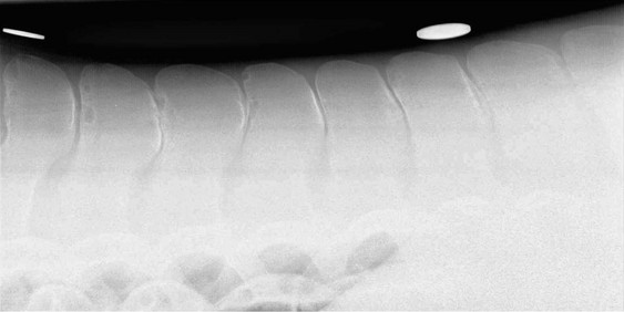
 The sheer size of an adult horse makes it impossible to get detailed radiographs of the abdomen. One exception where abdominal radiographs may be useful is to visualize the presence of sand or enteroliths in the gut.
Indications for radiography in the horse
Interpretation of radiographs
 Detection of obvious lesions distracts from other more subtle lesions.
 Pathological changes are mistaken for normal anatomical variation or artefact.
How to view radiographs?
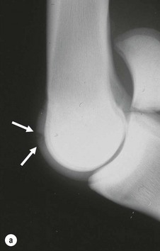
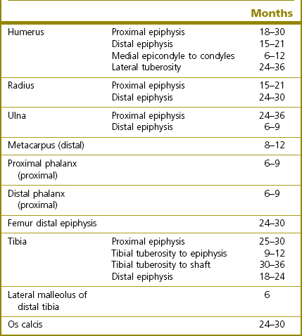
How to assess radiographs?
 Labelling: case number or name, date of examination, left–right, front–hind (necessary for projections distal to the carpus/tarsus), projections (including direction and degree of obliquity).
 Positioning/centring: is the area of interest on the radiograph?
 Sufficient number of views, additional projections required?
 Artefacts: movement, processing artefacts etc.
 Radiodensity: lucency versus opacity (opacities can be further categorized into soft tissue, mineral (often bone), metal density).
 Shape (spherical, elliptical, cylindrical, etc.).
 Margination (discrete, well/ill-defined or demarcated etc.).
Radiographic changes associated with musculoskeletal problems
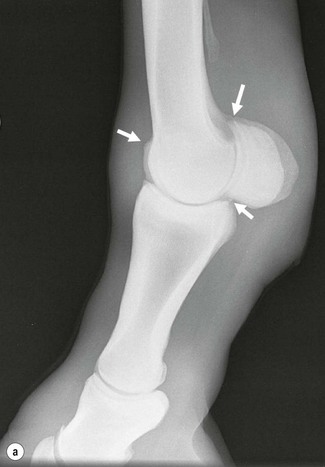
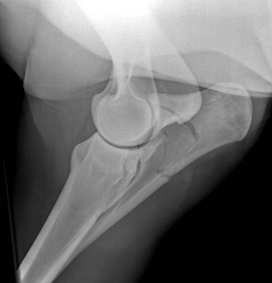
Osteoarthritis (Figures 25.4, 25.6, 25.7)
 Joint effusion: soft-tissue swelling around the affected joints.
 Periarticular osteophytes: new bone formation at the articular margins.
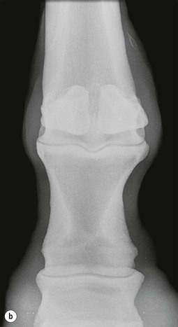
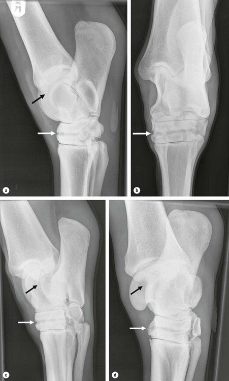
Osteochondrosis (Figures 25.10, 25.11)
 Changes in contour of bone surface (Figures 25.10a, 25.11a), most commonly flattening or depression, e.g. trochlear ridges of the talus or femur, humeral head.
 Subchondral bone sclerosis: on its own or in association with any of the other signs (Figure 25.11a,b).
 Subchondral bone lucency: focal or along the joint surface.
 Fragments: solitary or multiple (Figures 25.7, 25.10b, 25.11b).
 Well-defined (semi) circular or oval shaped lucency.
 Often surrounded by a sclerotic ring.
 Most commonly seen in the subchondral bone; however, may also be seen away from the joint.
 A neck-like connection between the cyst and the joint surface may be present.
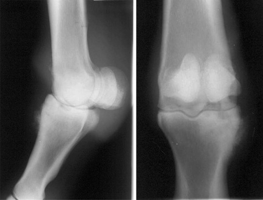
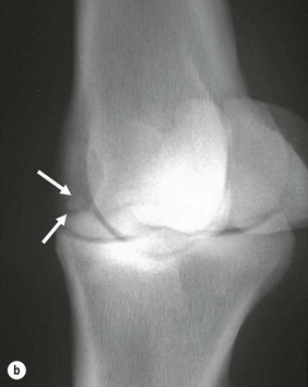
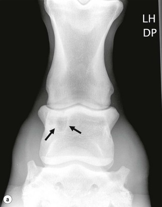
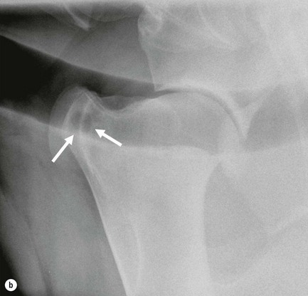
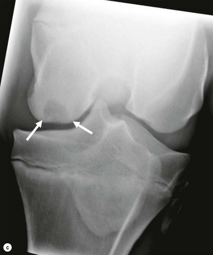
Infectious osteitis and osteoarthritis (Figure 25.1)
 Severe soft-tissue swelling around the affected area.
 Aggressive periarticular new bone production.
 Bone lysis characterized by irregular, poorly defined lytic areas.
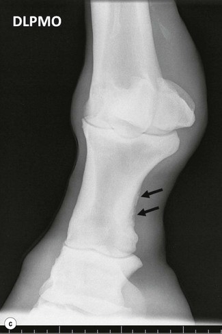
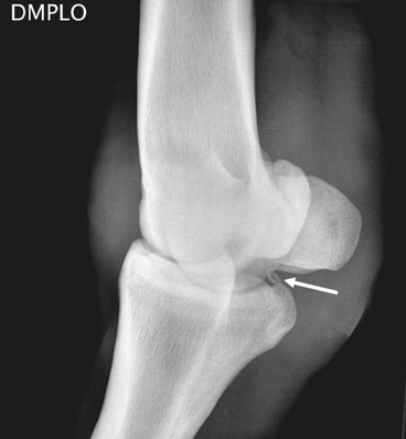
Enthesiopathies (Figures 25.5, 25.6)
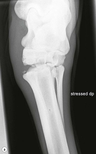
(Sub)luxations (Figure 25.13)
Fractures
 Is the fracture complete? The fracture line will extend from one end of the bone to the other. A single plane, complete fracture will appear as two lucent lines where the fracture plane traverses the two cortices!
 Is it a simple or comminuted fracture and if so how many separate fragments are there?
 Is the fracture displaced? This will lead to a disruption of the continuity of the bone surface.
 Does the fracture involve a joint? The fracture line will extend into one or two joints.
 Is the fracture open? Communication with the outside and/or soft tissue disruption will be visible.
 Long bone fractures (Figure 25.14).
 Condylar fractures (Figure 25.15).
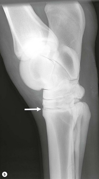
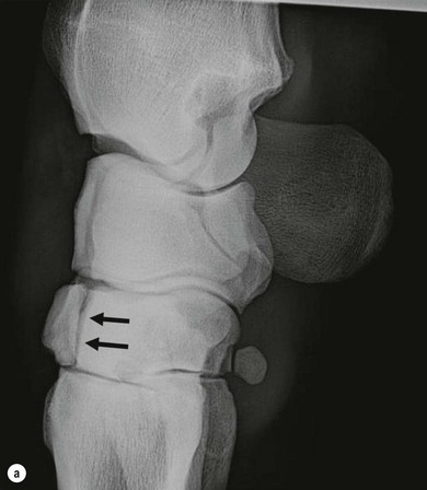
 Slab fractures: extend from one articular surface to the other, in carpal and tarsal bones (Figure 25.16).
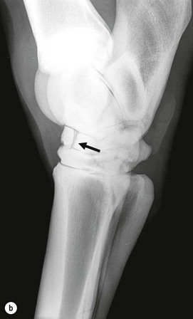
 Chip fractures: small fragments on articular margins (Figure 25.17).
 Avulsion fractures: at the attachment site of a ligament, tendon or muscle.
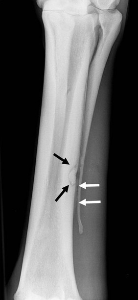
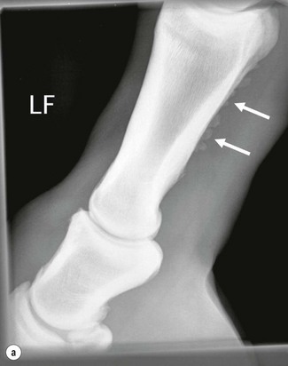
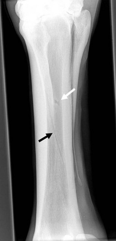
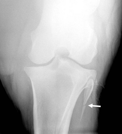
 Mach lines: these are radiolucent lines resulting from enhancement at the edge of two superimposed structures, e.g. the splint bones over the cannon bone (Figure 25.2).
 Nutrient foramina: these are usually wider than fracture lines and in known locations (Figure 25.19).
 Vascular channels in the distal phalanx (Figure 25.20).
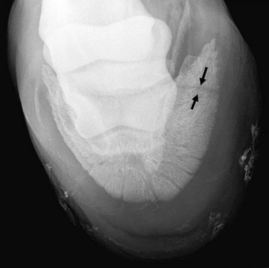
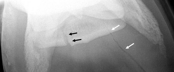
 Frog clefts, especially when they are inadequately packed: these usually extend beyond a single bone (Figure 25.21).
 Radiolucent lines between separate centres of ossification, especially fibula and hoof cartilages (Figure 25.22).
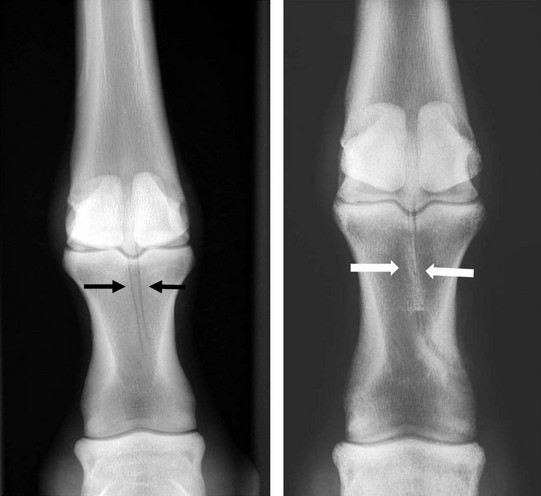
 Non-displaced fissure fractures may not be radiographically visible at first and scintigraphy is indicated in horses where a fracture is suspected, but cannot be visualized radiographically. Alternatively, the radiography can be repeated after 7–10 days (Figure 25.18).
 Callus: develops within 14–20 days of injury, often requires lower exposures for optimal visualization, fracture lines are less distinct and the fracture gap becomes narrowed and more radio-opaque.
 Fractures are often radiographically still visible while the fracture is already stable.
 A delayed union is present if a fracture line persists longer than 6 months.
 Soft-tissue calcification in the horse is usually secondary to soft-tissue injury causing haemorrhage and/or inflammation, e.g. suspensory ligament injuries.
 While plain radiographs are not very good in differentiating between soft-tissue densities, contrast radiographs are very useful in the evaluation of soft-tissue injuries because they can show the extent of the wound and the involvement of synovial structures.
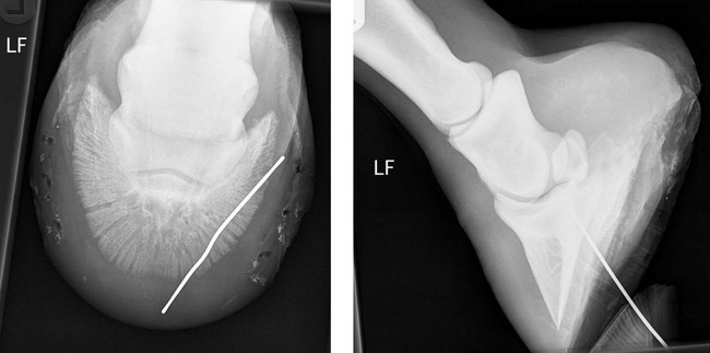
 A metal probe can first be inserted to assess the direction and depth of the wound. Two radiographs at 90° to each other are necessary to allow the visualization of the metal probe in 3D (Figure 25.23).
![]()
Stay updated, free articles. Join our Telegram channel

Full access? Get Clinical Tree