Fig. 1.
Diagram of an optical workstation utilizing Prairie View (Prairie Technologies, Inc.) and Win Fluor (University of Strathclyde) software. The movement and gain of the imaging laser is controlled using the commercially provided software Prairie View. Electrophysiological recordings are made using the free software package WinFluor, which is also used to control the position, timing, and gain of the photolysis laser. Imaging and physiological data are coordinated and displayed by WinFluor.
Two-photon excitation imaging of fluorescent dyes and indicators is most often performed with laser systems having pulse durations from 70 to 140 fs. The restriction of photon delivery in time, via mode-locking, increases the peak laser power at the sample plane, increasing the probability that an individual molecule will experience two-(or more) photon excitation. The advantage of nonlinear excitation is the restriction of fluorophore excitation to the focal volume determined by the objective lens. This allows optical sectioning (12). This mode of fluorescence excitation can greatly reduce background excitation and improves efficiency by permitting the collection of any emitted photons generated by the sampled probe. Thus, it does not require spatial filtering with a confocal pinhole aperture (which can reduce in-focus signal), since the emission signal collection is decoupled from the excitation event. This permits the collection of some of the emitted photons that are scattered while leaving the focal volume deeper into the brain slice tissue, increasing the detection sensitivity (13). Large front element objective lenses have an advantage in collecting this scattered signal – as long as the detector optical path is engineered to take advantage of the larger angles leaving the back of the objective lens (14). To effectively take advantage of this, two-photon imaging requires separate detectors optimized for full field emission collection.
1.2 System Components
In its simplest form, an optical experimental system is composed of a probe, an interaction, and an observation. A generic two-photon imaging system has been well described previously (12). This chapter briefly covers the basic components: laser, modulator, scanning mirrors, objective lens, optical filters, and detectors, as well as the optical workstation approach. How the first three items (laser, modulator, and mirrors) can be doubled and combined to add a second scanning channel for photo-stimulation and/or photolysis is also described.
1.2.1 Probe
The probe can be considered to be the laser and the instruments used to control the laser exposure and location. The laser most often employed is one with a Ti:Sapphire-based crystal laser with solid state 532 nm pump laser. Electro-optical modulators (Pockels cells) are used to control laser intensity since they have a very broad excitation wavelength range (700–1,200 nm) with low insertion loss (5%), rapid control (∼5 μs), the laser beam is not diverted by the Pockels cell and it requires no special lenses. If possible, the average laser power should be reduced to 1.5 W before the beam reaches the Pockels cell, as this greatly reduces heating load during imaging. However, newer lasers far exceed these average powers over most of the tuning range (<900 nm). A solution to this problem (employed by Prairie Technologies and in our lab) is the addition of a manual attenuator in front of the Pockels cell, which includes a rotating achromatic half-wave plate and fixed polarizing beam splitter cube. The cube permits sharing of the laser beam (at 90°) between two different scanning systems. Systems with this manual modulator scheme should keep both arms at 50% power to avoid polarization changes at the down-stream modulator(s). For average powers higher than 1.5 W, the best strategy is to leave the laser shutter open and place a mechanical shutter after the Pockels cell to aid modulator thermal equilibrium.
Cambridge galvanometer mirror systems, which allow manipulation of the laser target location in the x and y directions, are used by most commercial laser scanning microscope companies. The microscopes used for electrophysiology in brain slice work are most often upright in nature and the objective lenses used are water-dipping style for enhanced free working distances (2–3.3 mm) permitting pipette access for patching.
1.2.2 Interaction
The interaction refers to the excitation of a biologically relevant fluorescent molecule by the laser. Fluorophores, or fluorescent proteins, have optimal excitation photon energies, defined as excitation cross-section spectra. There is an inverse linear relationship between the photon wavelength and energy. The quantum mechanical selection rules for two-photon absorption events must be different from single photon absorption, so the energy levels involved will also be different. The rule in practice is to double the single photon spectra and then investigate lower wavelengths, higher photon energies. The ability to excite tissue with deep penetrating low-energy long wavelength light is a major advantage of 2P microscopy. For large symmetric molecules (like GFP), the two-photon cross-section spectra resemble the single photon spectra doubled. This is not true for second and third harmonic imaging, a scattering technique where the photon energy and momentum are conserved. In our experience, 820 nm photons work very well for most green-emitting fluorescent calcium indicators and ∼780 nm photons will optimally excite red Alexa-488, -568, and -594 dyes.
1.2.3 Observation
The strategies of dealing with the observation are the main focus of the remainder of this chapter. This includes collecting, interpreting, and displaying the experimentally collected photons in a biologically relevant way.
1.2.4 Limiting Phototoxicity
When working with living tissue, it is imperative to avoid inducing phototoxicity. As discussed below, in addition to frank distortions in structure, phototoxicity may also lead to more subtle changes in function, which may be overlooked during conventional physiological or anatomical experiments. Hence, great care must be taken in minimizing the stimulation exposure dose. The stimulation exposure dose is defined by the 2P excitation potential (power and space) multiplied by the duration of exposure (time). The excitation potential depends primarily on the square of the sample average power and linearly on the laser wavelength, as these are the two laser variables that historically have been the easiest to vary. Newer Ti:Sapphire lasers (Spectra Physics DeepSee and Coherent Vision) can now also control the pulse duration at the sample plane, so minimal average power can be used for a given stimulation dose. The signal obtained from 2P stimulation can be defined by the equation:
 where N is photon counting scans, t d is a time constant, n is the optical index of refraction of the immersion media, λ is the wavelength, g 2,p is a constant defining the laser pulse shape, R is the laser pulse repetition rate, τ is the pulse duration, P is the power, C represents the fluorophore concentration, σ 2 is the 2PEF cross section, and φ represents the fraction of light collected assuming isotropic emission.
1.3 Photo-Stimulation and Photolysis
Optical workstations can be modified to permit focused laser stimulation or 2PLU during imaging. Combining two-photon laser uncaging (2PLU) with 2PLSM increases system cost and requires a second ultra-short pulse duration laser (∼720 nm). In an attempt to minimize cost, lower power (10 W pump) laser systems or refurbished lasers have been used to power the 2PLU channel. Unfortunately, more affordable (compact, lower power) single-wavelength ultra-short pulse duration laser systems are not available with spectra near 700 nm (15). A more comprehensive set of criteria for selecting ultra-short pulse duration lasers for multiphoton excitation imaging can be found elsewhere (16).
The average powers reaching the sample (with a 60×, 0.9 NA objective) rarely approach 30 mW with 1 ms exposures, so very little of the full laser power (∼600 mW or more) is actually used for successful 2PLU with brain slices. The average photolysis laser power is attenuated with a Pockels cell, in the same manner as the imaging laser power. Great care must be taken with the modulator bias setting to ensure the best minimum (lowest power) to the sample plane. This minimizes photolysis during the “off” times of the stimulation protocol.
Despite the fact that the doubled one-photon excitation wavelength of 4-methoxy-7-nitroindolinyl (MNI)-glutamate (caged glutamate) is 630 nm, most applications of 2PLU to date have been done with Ti:sapphire lasers, which restricts the lower wavelength to 680 nm or 720 nm (depending on the laser pump power). The wavelength we use for 2PLU of MNI-glutamate is 720 nm. This wavelength is a compromise between the older, lower power laser systems (the manually tuned, 5 W pumped two-box lasers: Verdi/Mira, Millenia/Tsunami) which often yielded low average powers below 720 nm, and the newer commercially available one-box lasers (Chameleon-210, MaiTai-XF -BB) which cannot tune below ∼715 nm. The new series of pumped lasers (Chameleon-Ultra, MaiTai-HP) now permit 2P photolysis with average powers down to 680 nm or 690 nm.
Typical photolysis exposure times vary from microseconds to several milliseconds. With the Prairie Ultima system, it is possible to stimulate six distinct points within 1 ms with exposure times of only 100 μs at each point. Exposures of 0.5–1 ms at each point are much more common for experiments in slices. Spatial calibrations within the imaged field of view are verified using standard test samples to match the marked points for photolysis mirrors (galvanometers) to the voltages for the corresponding image pixel locations.
2 Imaging Applications in Brain Slices of the Basal Ganglia
2.1 The Challenge
The striatum is a complex subcortical nucleus that is populated by two major classes of spiny projection neurons (SPNs) and at least four classes of interneurons (2, 17–19). While this rich milieu undoubtedly increases the computational power of the striatum, it has traditionally posed severe constraints on the interpretation of physiological data collected in brain slices. There are three major obstacles. First, unlike other brain regions such as the cortex, hippocampus, and cerebellum, there is no obvious laminar organization in the striatum allowing positional identification of cell types (17). Moreover, with the exception of giant cholinergic interneurons, cell types are very difficult to visually distinguish using the IR-DIC optics typically used for patch-clamp recordings made in slices. Second, the two classes of SPN (which constitute ∼90% of all striatal neurons) are difficult to unequivocally distinguish either anatomically or physiologically (2, 17, 18, 20). Although there are differences (21–24), they are not so pronounced that they allow cells to be readily sorted in a patch-clamp experiment. Third, although interneurons can typically be identified by their physiological properties, they are extremely rare (constituting a few percent of all the neurons), making them difficult to find using standard IR-DIC optics (25, 26).
The recent development of BAC transgenic mice expressing fluorescent proteins under the regulation of cell-type specific promoters has offered a means of identifying specific striatal neuron populations (22, 27, 28). As mentioned above, striatal SPNs come in two major flavors: those primarily expressing D1 type dopamine receptors and projecting to the substantia nigra and internal globus pallidus (direct pathway) and those expressing D2 type dopamine receptors and projecting to the external segment of the globus pallidus (indirect pathway) (2, 18, 20, 29). These direct pathway SPNs (dSPNs) and indirect pathway SPNs (iSPNs) have similarly sized somata and spiny dendritic arbors that extend similar radial distances. With the advent of mice expressing GFP under the control of the D1 (BACD1) or D2 (BACD2) promoters, these two cell types can readily be distinguished (23, 27, 28). BAC transgenic mice expressing GFP or tdTomato reporters under the control of appropriate promoters can also be used to readily identify interneurons in brain slices. For example, mice expressing GFP under the control of parvalbumin or other cell-type specific promoters have been used to quickly sample from cholinergic, fast-spiking GABAergic and persistent low-threshold spiking interneurons in the striatum (30, 31).
2.2 Probing SPN Dendritic Anatomy
Traditionally, the dendritic anatomy of a neuron subjected to physiological interrogation was capable of being visualized only by filling the neuron with dye or another reactive molecule (e.g., biocytin), and then fixing, processing, and sectioning the slice after the experiment. 2PLSM has changed this situation and allows visualization of dendrites during the physiological experiment. By filling the patch electrode with a fluorophore (most commonly Alexa 568 or Alexa 594; 50 μM) that readily diffuses into the soma and dendrites, the entire dendrite can be visualized (27, 32, 33). Once the fluorophore has equilibrated throughout the dendritic tree (10–20 min post patching), the dye can be imaged. Imaging can be performed simultaneously with physiological somatic recordings if desired, in part because of the lower energy exposure to the slice afforded by the reliance upon longer wavelength 2P excitation.
2.2.1 The Z-Stack
Because 2P excitation is limited to a small focal volume in the specimen, anatomical data is collected in the form of an optical section in the z-axis. These optical sections can then be assembled into a stack (z-stack) to provide a three-dimensional image of the neuron (Fig. 2a, b). The lens used to acquire a z-stack should be of sufficiently high numerical aperture (NA) to resolve fine dendritic detail, but with a field of vision capable of capturing a sufficient portion (ideally all) of an average SPN dendritic field diameter. Larger NAs allow greater photon collection and therefore increased sensitivity. However, high NA typically decreases the working distance, making patch clamping difficult. We have found that a 60×/1.0 N.A. Olympus LUMPFL water-dipping lens is a reasonable compromise.
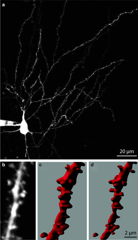
Fig. 2.
Reconstructing a 3D image of an SPN. (a). Maximum intensity projection image of an iSPN loaded with Alexa 568. (b) High zoom (4.9×) MIP of an iSPN dendrite. (c) 3D rendering of the dendrite shown in (b) using Imaris software to construct an isosurface from a nondeconvolved z-series. (d) 3D rendering of the same dendrite in (b, c) following a 60-cycle blind deconvolution of the z-series using AutoQuant. Scale bar in (d) applies to (b, d).
Once the lens is selected and the neuron patched and loaded with dye, there are five major variables that should be maximized to yield the highest quality z-stack.
1.
The digital zoom should be adjusted to include the appropriate field of view. While digital zoom is not needed for a whole cell image, it is an important variable to adjust when taking high magnification images of dendritic regions.
2.
The z-direction step size must be determined, and the z-direction limits defined. The step size should be small enough to pick up subtle anatomical features, yet not so small that the imaging time is increased unnecessarily. It should be noted that the ultimate maximal resolution is determined by the optics and laser properties given by
![$$ \begin{array}{lll} {\omega_{xy}} = \frac{{0.325\lambda }}{{\sqrt {2} {\text{N}}{{\text{A}}^{0.91}}}}, \hfill \\ {\omega_z} = \frac{{0.532\lambda }}{{\sqrt {2} }}\left[ {\frac{1}{{n - \sqrt {{{n^2} - {\text{N}}{{\text{A}}^2}}} }}} \right], \hfill \\ \end{array}, $$](/wp-content/uploads/2016/07/A210946_1_En_10_Chapter_Equb_10.gif) where NA is the numerical aperture of the lens (and is >0.7), λ is the wavelength of the excitation laser, and n is the refraction index of the immersion medium (12) and cannot be exceeded by altering the step size. We typically adjust our step size to be approximately one-half to one-third of the estimated z-plane resolution, in accordance with standard sampling theories. In addition to the step size, the top and bottom limit planes must be defined. This is done on a cell-by-cell basis.
where NA is the numerical aperture of the lens (and is >0.7), λ is the wavelength of the excitation laser, and n is the refraction index of the immersion medium (12) and cannot be exceeded by altering the step size. We typically adjust our step size to be approximately one-half to one-third of the estimated z-plane resolution, in accordance with standard sampling theories. In addition to the step size, the top and bottom limit planes must be defined. This is done on a cell-by-cell basis.
3.
The dwell time (amount of time the laser resides on each acquired pixel) should be adjusted to provide high enough photon emission to yield a quality image without increasing imaging time more than necessary. In our experiments, a dwell time of 4–10 μs is typically a good compromise.
4.
As all emitted photons are collected by the photomultiplier tubes (PMTs), it can be helpful to utilize averaging as a means of increasing signal-to-noise ratio (even though the signal-to-noise ratio is already vastly improved by 2PLSM compared to epifluorescence and confocal imaging (13)). To achieve this, multiple images can be taken at each focal plane and averaged.
5.
Finally, the laser sample power should be set to achieve an optimal signal-to-noise ratio for each cell. We achieve this through the use of a Pockels cell. As the image intensity diminishes as the image plane moves deeper into the slice, it is useful to increase the laser power with focal depth. This can be easily achieved with commercially available software. With the exception of setting the upper and lower focal plane limits and sample laser power, all of these steps can be standardized between neurons.
2.2.2 Deconvolution
Because the region of 2P excitation is not a single point and emitted photons are subject to diffraction by the slice, there is blurring of the acquired image. In general, 2P imaging greatly reduces blurring, as compared to confocal imaging, because of the tighter localization of the excitation volume. For instance, the optical setup in our laboratory yields a theoretical lateral resolution of 0.38 μm but an axial resolution of 1.43 μm. Blurring is most pronounced in the z-direction, because the 2P excitation region is maximally distorted in this direction. The process of removing out-of-focus signal is called deconvolution or deblurring (34, 35). The amount of blurring is directly related to the point spread function (PSF) of the imaging device. Deconvolution methods are implemented as iterative algorithms that consider an experimentally derived PSF and use a maximum likelihood estimator to minimize Poisson-distributed noise during each pass. Although the PSF can be measured and used during the deconvolution process, it is difficult to measure in real biological samples. Instead, blind deconvolution algorithms initially estimate and then refine the PSF during successive iterations (36). This function can be performed in a nearly automated fashion by commercially available software (described later). The benefits of deconvolving an image are most noticeable along the z-axis (Fig. 2c, d).
2.2.3 Direct Volume Rendering
Rendering techniques can be used to visualize the acquired and deconvolved dataset. Volume rendering is the process of creating a 2D image directly from a 3D image dataset, in this case, a series of slices that constitute a z-stack or from an intermediate 3D representation of the image data. When generating an image directly from image data, rays are cast from each point in the output image through the data (37). Samples are taken at discrete intervals along the ray usually using trilinear interpolation. The samples are used to determine a pixel’s final value (Fig. 3). In the simple case of a maximum intensity projection (MIP), the largest sample value along the ray is used to determine the pixel value. More complex compositing methods consider the contribution of all samples along a ray (38).
Fig. 3.
Volume rendering using ray casting. A ray starting at a point on the image plane is cast through the volume. Samples are taken at evenly spaced intervals along the ray. Because the data are discrete, trilinear interpolation is used to determine the value at each sample location.
In order to increase performance, isosurfaces or contour plots are often used as an intermediate representation (Fig. 2c, d). A 3D model is generated over a specified intensity value in the data, usually using the marching cubes algorithm (39). This computationally intensive operation is performed only once before rendering occurs, and generates a smaller, easier to render set of geometric primitives.
Most current volume rendering software takes advantage of the 3D texture mapping capabilities (40) of commonly used computer graphics cards. 3D texture mapping methods upload an entire volume dataset into a graphics card’s memory. Sampling using trilinear interpolation, and the application of color and opacity maps are performed entirely on the graphics card. This provides for great performance gains as long as the complete dataset fits in the graphics card’s video RAM.
Rendering and viewing the reconstructed dataset allows for cursory visual inspection and estimates of dendrite length and spine number and types. More sophisticated software packages use image segmentation and computational geometry techniques to automate 3D dendrite tracing, branch detection, and spine counting. These programs can further categorize spines into defined shapes (i.e., mushroom, stubby, thin), which have been correlated with various states of synaptic plasticity (41–44). A number of software packages (commercial and free) exist that aid in the anatomical reconstruction and analysis of neurons. Volocity (PerkinElmer, Inc.) and Amira (Visage Imaging, Inc.) are commercial products that offer deconvolution, rendering, and image analysis features. Imaris (Bitplane, Inc.) is a rendering and analysis package aimed specifically at cellular and neuronal applications, and integrates with the AutoQuant/AutoDeblur (Media Cybernetics, Inc.) deconvolution package. NeuronStudio (Mount Sinai School of Medicine), Voxx (Indiana University), and NUPVer (Northwestern University) are free applications that have simple rendering and measurement tools. Kitware, Inc. maintains popular open source C++ software libraries for visualization, rendering, and image analysis, including the Visualization Toolkit (VTK) (http://www.vtk.org), and the National Library of Medicine’s Insight Segmentation and Registration Toolkit (ITK) (http://www.itk.org). Even with these rather advanced tools, deconvolution and rendering can take many hours or even days on current workstations. A typical z-series spanning 200 × 200 × 100 μm and sampled with a pixel size of 0.36 μm and z-step of 0.2 μm can take up to half a GB. Large datasets also pose a challenge for fully automated analysis packages. Computationally complex tasks, such as spine counting, have not been successfully automated to date (at least not in our hands).
2.2.4 Limitations
While 2PLSM offers striking benefits for analyzing neuronal anatomy, there are several caveats. One caveat is that the neuronal properties might change during the time it takes to dialyze the cell and acquire an image. For SPNs, the cell must load with dye for 10–20 min before a z-stack can be made and each stack can take up to 20 min to complete. Another caveat is that if the slice physically moves, the acquired image will be distorted. Furthermore, image quality will be inversely related to their depth in the slice. This limitation is worsened by the fact that emitted photons are typically of shorter wavelength than the exciting photons, resulting in greater diffraction. As a consequence, cells chosen for imaging must not be too deep (typically no deeper than 80 μm below the surface). Dendrites descending deep into the slice, though equally likely to fill with the added fluorophore, will not be detected as efficiently. This is a real problem with SPNs, as they have spherical dendritic trees (3, 45, 46). Finally, as the optical density of brain tissue typically increases with age (45), imaging neurons in brain slices from older mice can be problematic and require adjustment of imaging conditions.
2.3 Dendritic Calcium Imaging
Compared to projection neurons in other brain regions, SPNs have very fine caliber dendrites. In fact, the distal tips of SPN dendrites have been estimated to be only about a third of a micron in diameter (3). As mentioned above, this makes direct patch clamping of distal dendrites virtually impossible with current methodologies. An alternative to direct voltage measurements is to measure calcium flux through voltage-gated calcium channels in neurons subjected to patch-clamp recording (27, 33, 47). Although there is a rough correlation between calcium entry and membrane voltage in many of the experimental situations we described, the two are not interchangeable and appropriate caution should be used in interpreting data. For example, cytosolic calcium transients may come not only from opening voltage-dependent channels in the plasma membrane, but also from intracellular sources that are not voltage sensitive (48–50). Nevertheless, the combination of electrophysiological and optical approaches has major strengths in studying neuronal properties. One of the challenges we have faced is the integration of electrophysiological and optical data acquisition modalities in the same workstation. Some of the solutions we have developed are discussed within the context of the methodology for dendritic calcium imaging.
2.3.1 Calcium Dye Selection
The most common method of imaging calcium transients in living tissue involves loading the cell(s) of interest with a calcium-sensitive indicator. This fluorophore must (1) have an appropriate affinity for calcium (as such, BAPTA/EGTA are typically the starting point for the indicator’s construction) and (2) be capable of changing its photon absorption or emission efficiency based on its binding state with calcium (51, 52). We only discuss imaging calcium signals using nonmembrane-permeable calcium dyes (free acids) loaded through the recording electrode. When collections of neurons are to be imaged, membrane permeable AM-ester modified dyes are a viable alternative, but these approaches are not discussed here (53–56).
The first step in designing a calcium imaging experiment is choosing an appropriate dye. Two factors should be taken into consideration when making this decision: the affinity of the dye for calcium and its absorption/emission spectrum. Calcium dyes have a wide range of affinities. Which dye is appropriate for a particular experiment will depend on the physiology of the cell type to be examined and the phenomenon to be studied. The dye should have a low enough calcium affinity that it does not disrupt basal cytoplasmic calcium signaling. Supplemental calcium buffers such as EGTA or BAPTA (which are commonly included in many internal recording solutions) should not be used in these experiments, as the calcium dye itself should be adequate to buffer calcium in the internal solution. The relationship between calcium binding and photon emission should be linear within the range of calcium concentrations being measured. In our experience, a high-affinity dye such as Fluo-4 is useful for studying calcium dynamics associated with modest physiological stimuli such as short trains of action potentials or excitatory postsynaptic potentials (EPSPs). Fluo-4 fluorescence is minimal in SPNs at resting membrane potentials (approximately −80 mV), and we have observed little evidence of dye saturation in most circumstances. The optimal concentration of Fluo-4 needed may differ between protocols. We typically find that 200 μM Fluo-4 provides a strong calcium signal without disrupting cellular function in any obvious way. It should be noted here that great care must be taken when choosing a dye and corresponding concentration when examining phenomena governed by calcium dynamics, as such events will be sensitive to exogenous buffering.
In addition to having an appropriate calcium affinity, the dye must also have 2-photon absorption/emission wavelengths appropriate for the equipment being used. Several criteria should be met by this choice:
1.


The maximum 2P excitation cross section should be readily achieved using the system’s laser (820 nm is fine for most green-emitting indicators);
< div class='tao-gold-member'>
Only gold members can continue reading. Log In or Register to continue
Stay updated, free articles. Join our Telegram channel
Full access? Get Clinical Tree
